python数据分析：使用statsmodels构建价格需求弹性模型

价格需求弹性（Price elasticity of demand）

是经济学中使用的一种衡量标准，用于显示商品或服务所需数量对价格变化的响应性或弹性，除了价格变化。更确切地说，它给出了响应价格百分之一变化所需数量的百分比变化。

在经济学中，弹性是衡量需求或供给对价格敏感程度的指标。
在营销中，消费者对产品价格变化的敏感程度如何。

它给出了以下问题的答案：

• “如果我降低产品的价格，还会卖多少钱？”
• “如果我提高一种产品的价格，这将如何影响其他产品的销售？”
• “如果产品的市场价格下降，那将影响公司愿意向市场供应的金额多少？”

数据

一份关于牛肉价格数量随时间变化的数据

数据描述

• Year：年份
• Quarter：季度
• Quantity：数量
• Price：价格

python实践

1.导入库 和 数据

import numpy as np
import pandas as pd
import matplotlib.pyplot as plt
import statsmodels.api as sm
from statsmodels.formula.api import ols
from statsmodels.compat import lzip
from __future__ import print_function

%matplotlib inline

df = pd.read_csv('https://raw.githubusercontent.com/ffzs/dataset/master/beef.csv')
df.head()

2.查看缺失值

# 检查缺失值，没有
df.isnull().values.any()

False

3.合并年和季度数据

# 年和季度合并
df['Year'] = pd.to_datetime(df['Year'], format="%Y")
from pandas.tseries.offsets import *
df['Date'] = df.apply(lambda x:(x['Year'] + BQuarterBegin(x['Quarter'])), axis=1)
df.drop(['Year', 'Quarter'], axis=1, inplace=True)
df.set_index('Date', inplace=True)

4.数据简单观察

# 简单观察数量和价格跟随时间的变化
df.plot.line(subplots=True)

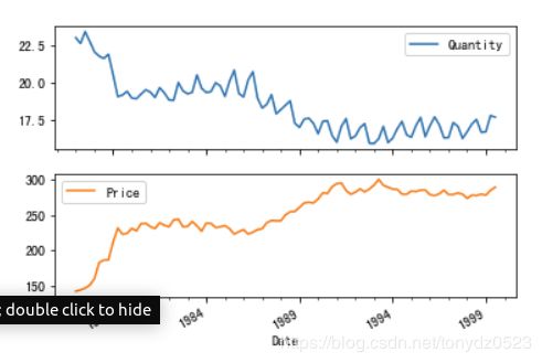
# 通过散点图简单看一下数量和价格之间的关系成负相关
df.plot.scatter(x='Quantity', y='Price', c='g', s=18)

回归分析

最小二乘法（Ordinary Least Squares）估计

# 获取自变量和因变量
x = df.Quantity
y = df.Price
X = sm.add_constant(x)

ols_model = sm.OLS(y, X)
result = ols_model.fit()

print(result.summary2())

结果如下：

可见：

• P值很小说明价格和数量无关的null hypothesis被拒绝
• 高R平方值也说明了我们的模型预测很准

展示图表用于更直观的解释回归分析

# 调出y的拟合值
y_fit = result.fittedvalues
# 使用matplotlib画图
fig, ax= plt.subplots(figsize=(10,6))
# 画图原始数据
ax.plot(x, y ,'o', label='raw_data')
# 画出拟合后的数据
ax.plot(x, y_fit, 'r--.',label='OLS')
#放置注释
ax.legend(loc='best')

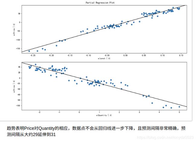
fig = plt.figure(figsize=(12,8))
fig = sm.graphics.plot_partregress_grid(result, fig=fig)

CCPP图

CCPR图提供了一种方法，通过考虑其他自变量的影响来判断一个回归量对响应变量的影响。

fig = plt.figure(figsize =(12,8))
fig = sm.graphics.plot_ccpr_grid(result,fig = fig)

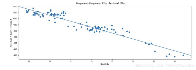
正如您所看到的，由Price解释的数量变化之间的关系是明确的线性。没有太多的观察结果对这种关系产生了相当大的影响。

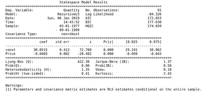
递归最小二乘（RLS）

最后，我们应用递归最小二乘（RLS）滤波器来研究参数不稳定性

endog = df['Quantity']
exog = sm.add_constant(df['Price'])
mod = sm.RecursiveLS(endog, exog)
res = mod.fit()
print(res.summary())

RLS图

我们可以在给定变量上生成递归估计系数图。

res.plot_recursive_coefficient(range(mod.k_exog), alpha=None, figsize=(10,6))

为方便起见，我们使用plot_cusum函数直观地检查参数稳定性。

fig = res.plot_cusum(figsize=(10,6))

在上图中，CUSUM统计量不会超出5％显着性带，因此我们未能拒绝5％水平的稳定参数的零假设。