摩拜单车骑行数据探索性分析【实战总结】

项目背景

项目背景：2017年biendata举办了摩拜杯算法挑战赛，利用机器学习去预测每个用户可能的骑行目的地，以更好地调配和管理大量摩拜单车。

数据下载地址：项目官网 https://biendata.com/competition/mobike/

本文将使用项目中给出的训练集数据train.csv进行数据的探索性分析，利用python工具来探索用户骑行规律。暂不涉及建模。

分析的目的：获取用户出行的规律，主要分析维度是时间，日期，骑行距离等

文中Geohash脚本 下载链接: https://pan.baidu.com/s/17J-22GdN4F2jEOxWPvQ-Eg 提取码: vhbz

工具：Jupyter notebook Python 3

数据概况

import pandas as pd
import datetime
import geohash
import seaborn as sns
import matplotlib.pyplot as plt
%matplotlib inline
from math import radians, cos, sin, asin, sqrt

# 导入train.csv数据文件,将starttime转换为日期列，避免后续字符串和datetime的转换
df = pd.read_csv("train.csv",sep=",",parse_dates=["starttime"])

# 查看数据集df
df.head()

	orderid	userid	bikeid	biketype	starttime	geohashed_start_loc	geohashed_end_loc
0	1893973	451147	210617	2	2017-05-14 22:16:50	wx4snhx	wx4snhj
1	4657992	1061133	465394	1	2017-05-14 22:16:52	wx4dr59	wx4dquz
2	2965085	549189	310572	1	2017-05-14 22:16:51	wx4fgur	wx4fu5n
3	4548579	489720	456688	1	2017-05-14 22:16:51	wx4d5r5	wx4d5r4
4	3936364	467449	403224	1	2017-05-14 22:16:50	wx4g27p	wx4g266

数据字段说明

• orderid 订单号
• userid 用户ID
• bikeid 车辆ID
• biketype 车辆类型
• starttime 骑行起始日期时间
• geohashed_start_loc 骑行起始区块位置
• geohashed_end_loc 骑行目的地区块位置

df.info()

RangeIndex: 3214096 entries, 0 to 3214095
Data columns (total 7 columns):
orderid                int64
userid                 int64
bikeid                 int64
biketype               int64
starttime              datetime64[ns]
geohashed_start_loc    object
geohashed_end_loc      object
dtypes: datetime64[ns](1), int64(4), object(2)
memory usage: 171.7+ MB

# 数据集大小 3214096 * 7
df.shape

(3214096, 7)

# 数据涵盖了48万+的单车
df.bikeid.unique().size

485465

# 数据涵盖了近35W的骑行用户
df.userid.unique().size

349693

# 涵盖2种车型
df.biketype.unique().size

2

# 查看geohashed_start_loc 字段长度
df["geohashed_start_loc"].apply(lambda s: len(s)).value_counts()

7    3214096
Name: geohashed_start_loc, dtype: int64

# 查看geohashed_end_loc 字段长度
df["geohashed_end_loc"].apply(lambda s: len(s)).value_counts()

7    3214096
Name: geohashed_end_loc, dtype: int64

查看整个数据情况，可了解到数据集大小为3214096 * 7，涵盖48W+单车、近35W骑行用户、2种单车车型。
骑行出发点、目的地经过Geohash编码加密，且全部为7位编码。

选取数据分析样本

考虑到数据集大小以及电脑的性能，同比例随机挑选50%的数据进行用户行为分析

df = df.sample(frac=0.5)

df.info()

Int64Index: 1607048 entries, 120096 to 241942
Data columns (total 7 columns):
orderid                1607048 non-null int64
userid                 1607048 non-null int64
bikeid                 1607048 non-null int64
biketype               1607048 non-null int64
starttime              1607048 non-null datetime64[ns]
geohashed_start_loc    1607048 non-null object
geohashed_end_loc      1607048 non-null object
dtypes: datetime64[ns](1), int64(4), object(2)
memory usage: 98.1+ MB

数据处理

时间处理

当前数据中只有骑行出发时间starttime，格式同 2017-05-14 22:16:50

时间进行处理，提取出周几weekday，小时hour，日期day数据，以便后续分析不同时间出行数据的分布

# 使用weekday函数提取周几信息，周一为0，周日为6
df["weekday"] = df["starttime"].apply(lambda s: s.weekday()) 

# 提取小时数，hour属性
df["hour"] = df["starttime"].apply(lambda s: s.hour)

# 提取时间中的日期
df["day"] = df["starttime"].apply(lambda s:str(s)[:10])

# 打印日志
print("时间信息处理完毕！")  

时间信息处理完毕！

空间信息处理

数据集中，地理位置通过Geohash加密，算法比赛的官网上告知可以通过开源的方法获得经纬度数据。

本文是直接导入Geohash脚本进行处理经纬度的处理

关于Geohash编码的原理，强烈推荐阅读此文：https://www.cnblogs.com/LBSer/p/3310455.html

Geohash感性认识：

• GeoHash将二维的经纬度转换成字符串，比如下图展示了北京9个区域的GeoHash字符串，分别是WX4ER，WX4G2、WX4G3等等，每一个字符串代表了某一矩形区域。这个矩形区域内所有的点（经纬度坐标）都共享相同的GeoHash字符串，这样既可以保护隐私（只表示大概区域位置而不是具体的点），又比较容易做缓存，比如左上角这个区域内的用户不断发送位置信息请求附近餐馆数据，由于这些用户的GeoHash字符串都是WX4ER，所以可以把WX4ER当作key，把该区域的餐馆信息当作value来进行缓存，而如果不使用GeoHash的话，由于区域内的用户传来的经纬度是各不相同的，很难做缓存。
  
• Geohash能够提供任意经度的分段级别，一般分为1-12级。Geohash编码字符串越长，表示的区域范围越精确。
  

前面已经验证过，数据集中Geohash区块位置信息全部为7位Geohash编码。按照对应的精度级别，每个区块在153米*153米范围内。G7位编码对应的区块范围很小，单车随意骑行，一般都能离开当前区域。

构建区块对应的6位Geohash编码，每个区块面积在1.22km*0.61km范围内，比较符合短途摩拜骑行的特点。

当然，我们还可以从7位Geohash编码中不断提取更短的编码进行研究分析，但建议到4位即可。
如果编码更短，比如3位，区块面积太大，就会变得没意义。

def geo_data_process(df):
    # 通过导入Geohash脚本中的decode函数，获取经纬度
    df["start_lat_lng"] = df["geohashed_start_loc"].apply(lambda s: geohash.decode(s))   
    df["end_lat_lng"] = df["geohashed_end_loc"].apply(lambda s: geohash.decode(s))
    
    #获取出发地点所在区块周围的8个相邻区块编码
    df["start_neighbors"] = df["geohashed_start_loc"].apply(lambda s: geohash.neighbors(s))
    
    # 提取区块对应的6位Geohash编码
    df["geohashed_start_loc_6"] = df["geohashed_start_loc"].apply(lambda s: s[0:6])
    df["geohashed_end_loc_6"] = df["geohashed_end_loc"].apply(lambda s: s[0:6])
    
    #获取出发地点所在区块周围的8个相邻区块的6位Geohash编码
    df["start_neighbors_6"] = df["geohashed_start_loc_6"].
    							apply(lambda s: geohash.neighbors(s))
    print("Geohash编码处理完毕！")    
    
    # 判断目的地是否在当前区块或相邻区块内
    def inGeohash(start_geohash,end_geohash,names):
            names.append(start_geohash)
            if end_geohash in names:
                return 1
            else:
                return 0 
    
    df['inside'] = df.apply(lambda s :inGeohash(s['geohashed_start_loc'],
    						s['geohashed_end_loc'],
    						s['start_neighbors']),
    						axis = 1)
    df['inside_6'] = df.apply(lambda s :inGeohash(s['geohashed_start_loc_6'],
    					    s['geohashed_end_loc_6'],
    					   	s['start_neighbors_6']),
    					   	axis = 1)
    print("判断目的地操作处理完毕!!!")
    
    # 用haversine公式计算球面两点间的距离
    def haversine(lon1,lat1,lon2,lat2):
        lon1,lat1,lon2,lat2 = map(radians,[lon1,lat1,lon2,lat2])
        dlon = lon2 - lon1
        dlat = lat2 - lat1
        a = sin(dlat/2)**2 + cos(lat1)*cos(lat2)*sin(dlon/2)**2
        c = 2 * asin(sqrt(a))
        r = 6371 # 地球平均半径，单位为公里
        return c * r * 1000

    df["start_end_distance"] = df.apply(lambda s : haversine(s['start_lat_lng'][1],
    									s['start_lat_lng'][0],s['end_lat_lng'][1],
    									s['end_lat_lng'][0]),axis = 1)
    print("两点距离计算完成!!!") 

geo_data_process(df)

Geohash编码处理完毕！
判断目的地操作处理完毕!!!
两点距离计算完成!!!

数据分析

时间分析

# 统计数据集中天数
print("数据集包含的天数如下：")
print(df["day"].unique())

数据集包含的天数如下：
['2017-05-16' '2017-05-20' '2017-05-18' '2017-05-19' '2017-05-12'
 '2017-05-11' '2017-05-13' '2017-05-14' '2017-05-24' '2017-05-15'
 '2017-05-21' '2017-05-22' '2017-05-10' '2017-05-23']

分析24小时骑行订单数分布情况：

hour_group = df.groupby("hour")
hour_group["orderid"].count().sort_values(ascending=False)

hour
7     157885
18    144791
8     142543
17    136779
19    104823
12    100368
16     89496
11     86010
13     81895
15     77576
20     75759
9      73782
14     68191
21     64042
10     63099
6      60914
22     35010
5      14489
23     14376
0       6524
1       3137
4       2216
2       1853
3       1490
Name: orderid, dtype: int64

从每小时订单数的降序排列中，发现排位在前面的时刻为7、18、8、17、19点，这些时间段是上下班高峰期，用户使用单车数量较多。
做出直方图，看整体趋势：

# 不同小时的出行量
hour_num_df = hour_group.agg({"orderid":"count"}).reset_index()
sns.barplot(x = "hour",y = "orderid",data =hour_num_df )

图形呈现出的变化更为直观！
23-5点这段时间，人们大多在休息，使用单车出行的订单数极少。
6点开始，活跃用户增多。在7-8点、17-18点上下班时段，单车订单量迅速增长，呈现明显的骑行早晚高峰。
11-13点时段，出现局部午高峰，这和中午外出就餐或者休息时间活动有一定关系。
整体趋势，说明单车的骑行交通在很大程度上是服务于通勤交通的。

如果是在周末，非工作日内骑行情况随时间的分布如何呢？
这里新增是否为周末的数据维度"isWeekend"，展开进一步探索。

# 区分是否为周末，增加维度"isWeekend"
df.loc[(df["weekday"]==5) | (df["weekday"]==6),"isWeekend"]=1
df.loc[~((df["weekday"]==5) | (df["weekday"]==6)),"isWeekend"]=0

# 计算工作日天数，周末的天数
w = df[(df["isWeekend"]==1) & (df["weekday"]>=5)]["day"].unique().size
c = df[(df["isWeekend"]==0) & (df["weekday"] <5)]["day"].unique().size

print("非工作日天数:",w)
print("工作日天数:",c)

非工作日天数: 4
工作日天数: 10

通过上面计算得到，整个数据对应的时间为 4个非工作日，10个工作日。
下面分别计算出工作日、非工作日每个小时的平均订单量，查看随时间变化的订单量分布情况。

g1 = df.groupby(["isWeekend","hour"])
temp_df = pd.DataFrame(g1['orderid'].count()).reset_index()
temp_df.loc[temp_df['isWeekend'] == 0.0,'orderid'] = temp_df['orderid'] / c
temp_df.loc[temp_df['isWeekend'] == 1.0,'orderid'] = temp_df['orderid'] / w
sns.barplot(x = 'hour',y ="orderid" ,hue = "isWeekend",data = temp_df )

isWeekend=0，蓝色柱状表示工作日内每小时平均订单量的分布。同上述每小时总订单量分布情况相似： 23-5点这段时间，使用单车出行的订单数极少。 6点开始，活跃用户增多。在7-8点、17-18点上下班时段，单车订单量迅速增长，呈现明显的骑行早晚高峰。 11-13点时段，出现局部午高峰。

isWeekend=1，橙色柱状为非工作日内每小时平均订单量的分布。周末骑行交通以非通勤交通为主，时间分布相对平缓，没有明显的早高峰现象。整体骑行订单量明显少于工作日的骑行订单量。

通过对比分析，摩拜单车最大使用量出现在工作日的上下班高峰。

出行时间、是否在双休日，这两个特征对骑行订单量有明显影响，反映出用户行为特点。

骑行距离分析

# 出行距离的描述统计
df["start_end_distance"].describe()

count    1.607048e+06
mean     8.150117e+02
std      6.888783e+02
min      1.163695e+02
25%      4.654801e+02
50%      6.603909e+02
75%      9.497557e+02
max      4.490018e+04
Name: start_end_distance, dtype: float64

上述描述统计值：用户骑行距离的平均值815米，中位数660米，75%在949米。这几个数据反映了用户一般为近距离骑行，比较合理。
但最大距离值达到44900米，初步判断应该是个异常值，一般人骑行不会骑这么远。

# 用户骑行距离分布图
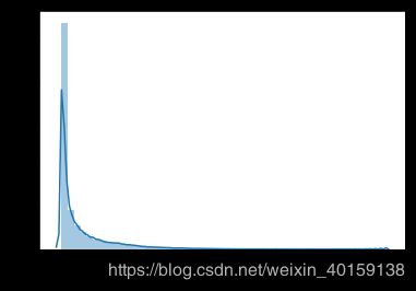
sns.distplot(df["start_end_distance"])

骑行距离分布图显示出主要的骑行距离大概集中在5000米范围内。但也存在远距离甚至40公里以上的骑行，考虑到定位问题存在一些特殊性，可考虑为异常数据；或者可以理解为其他特殊的骑行现象。

将5000米骑行距离外的数据做进一步剔除，再做一层过滤，更清晰地观察骑行距离的分布。

# 剔除一些极端的骑行距离案例
start_end_distance = df["start_end_distance"]
start_end_distance = start_end_distance.loc[start_end_distance<5000]
sns.distplot(start_end_distance)

剔除5000米以上距离的数据后，骑行距离的分布可以看得更明显了。大部分用户骑行距离还是在1000米内的。
当然，还可以重复上述操作，继续缩小距离到4000米，3000米，会更清晰地查看分布！

通过前面的分析，时间对骑行订单量的分布有明显影响。那么，时间对骑行距离是否也会产生影响呢？
接着分析不同时间段的平均骑行距离。

# 不同时间段的骑行距离
hour_group = df.groupby("hour")
hour_distance = hour_group.agg({"start_end_distance":"mean"}).reset_index()
sns.barplot(x='hour',y='start_end_distance',data=hour_distance)

图形反映出随时间的变化，骑行距离变化趋势较为平缓，可理解为骑行时间对骑行距离不会产生太大影响。

另外，数据集中给出了两种摩拜单车的车型，车型是否对骑行距离有影响呢？
查看车型对应的用户平均骑行距离。

# 摩拜单车分为1代，2代两种车型，分析两种车型的平均骑行距离
g_biketype = df.groupby("biketype")
g_biketype.agg({"start_end_distance":"mean"})

	start_end_distance
biketype
1	808.862414
2	824.435284

两代车型的骑行距离没有太大区别，平均骑行距离都在800米左右，不同的车型对骑车距离没有影响。

用户出发地与目的地分析

分析出发点或到达点每天对应的用户量、车辆数量、订单量分布

def analysis_1(data,target):
    g1 = data.groupby(["day",target])
    group_data = g1.agg({"orderid":"count","userid":"nunique",
						"bikeid":"nunique"}).reset_index()
    for each in ["orderid","userid","bikeid"]:
        sns.distplot(group_data[each])
        plt.show()
    return group_data

group_data = analysis_1(df,"geohashed_start_loc")

上面生成的3个图形，是根据出发点“geohashed_start_loc”计算出的用户量、订单量、单车量的分布。

数量集中在偏向0的位置，说明每个出发点匹配到的用户数量、单车量、订单量都很少。

使用describe()函数，查看各项统计值。

group_data.describe()

	orderid	userid	bikeid
count	483885.000000	483885.000000	483885.000000
mean	3.321136	3.239700	3.306496
std	4.811719	4.722345	4.776035
min	1.000000	1.000000	1.000000
25%	1.000000	1.000000	1.000000
50%	2.000000	2.000000	2.000000
75%	4.000000	4.000000	4.000000
max	154.000000	152.000000	153.000000

每个区块仅平均匹配到3个订单，3个用户，3辆车。25%，50%，75%分位数同样说明了出发点匹配到的骑行相关数量是很少的。
因为这里是按照7位Geohash编码计算的分布情况。考虑到7位编码对应的区块面积非常小，骑行数量很少也不难理解。

如果换位6位编码，区域面积放大，是否订单量、用户量、车辆数都会变化呢？

group_data_6 = analysis_1(df,"geohashed_start_loc_6")

可以明显看出数量范围变大了，用describe函数看统计信息

group_data_6.describe()

	orderid	userid	bikeid
count	56959.000000	56959.000000	56959.000000
mean	28.214119	26.145736	27.414754
std	48.636984	45.326965	46.978754
min	1.000000	1.000000	1.000000
25%	2.000000	2.000000	2.000000
50%	7.000000	6.000000	6.000000
75%	32.000000	29.000000	31.000000
max	546.000000	527.000000	528.000000

每个6位Geohash编码区块中平均产生28个订单，有26个用户，27辆车。

我们可以想象，如果将编码长度继续缩小，对应的订单量等也会相应地变大。

将数据按照日期，出发点、目的点进行分组，统计各记录匹配到的用户量、订单量、单车量、以及平均骑行距离

# 计算 出发点-目的点 的 订单量，车辆数，用户数
start_end = df.groupby(["day","geohashed_start_loc","geohashed_end_loc"])
start_end.agg({"orderid":"count","userid":"nunique","bikeid":"nunique",
				"start_end_distance":"mean"}).reset_index().
				sort_values(by = "orderid",ascending = False)

	day	geohashed_start_loc	geohashed_end_loc	orderid	userid	bikeid	start_end_distance
172759	2017-05-11	wx4f9ky	wx4f9mk	40	38	40	385.045143
290218	2017-05-12	wx4f9ky	wx4f9mk	37	36	37	385.045143
743058	2017-05-16	wx4f9ky	wx4f9mk	33	32	33	385.045143
875354	2017-05-18	wx4f9ky	wx4f9mk	33	33	33	385.045143
1011883	2017-05-19	wx4f9ky	wx4f9mk	30	30	30	385.045143
619106	2017-05-15	wx4f9ky	wx4f9mk	30	29	30	385.045143
875309	2017-05-18	wx4f9kn	wx4f9ms	28	28	28	945.750759
503803	2017-05-14	wx4f9ky	wx4f9mk	28	28	28	385.045143
102471	2017-05-10	wx4gd3e	wx4gd91	28	28	28	765.452392
56190	2017-05-10	wx4f9ky	wx4f9mk	28	28	28	385.045143
290336	2017-05-12	wx4f9mk	wx4f9ky	27	27	26	385.045143
875483	2017-05-18	wx4f9mk	wx4f9ky	27	27	27	385.045143
56310	2017-05-10	wx4f9mk	wx4f9ky	27	26	27	385.045143
743020	2017-05-16	wx4f9kn	wx4f9mk	26	26	26	798.714812
1012006	2017-05-19	wx4f9mk	wx4f9ky	26	26	26	385.045143
619252	2017-05-15	wx4f9ms	wx4f9ky	25	25	25	514.635486
743176	2017-05-16	wx4f9mk	wx4f9ky	24	24	24	385.045143
187689	2017-05-11	wx4fg87	wx4ferq	24	24	24	846.527290
619213	2017-05-15	wx4f9mk	wx4f9ky	23	23	22	385.045143
744399	2017-05-16	wx4f9wb	wx4f9mu	23	23	23	770.061723
618122	2017-05-15	wx4f94q	wx4f94t	23	3	22	192.537565
503902	2017-05-14	wx4f9mk	wx4f9ky	22	21	22	385.045143
172890	2017-05-11	wx4f9mk	wx4f9ky	22	22	22	385.045143
172727	2017-05-11	wx4f9kn	wx4f9mk	22	22	22	798.714812
1011848	2017-05-19	wx4f9kn	wx4f9ms	22	22	22	945.750759
1329605	2017-05-23	wx4f9ky	wx4f9mk	22	22	22	385.045143
875308	2017-05-18	wx4f9kn	wx4f9mk	21	21	21	798.714812
716408	2017-05-16	wx4eq0c	wx4eq23	21	21	21	985.047239
219987	2017-05-11	wx4gd3e	wx4gd91	21	21	21	765.452392
1068753	2017-05-19	wx4ghcm	wx4ghc8	21	21	19	605.232188
...	...	...	...	...	...	...	...
496796	2017-05-14	wx4f6dt	wx4f6e5	1	1	1	385.162205
496795	2017-05-14	wx4f6dt	wx4f6du	1	1	1	192.581816
496794	2017-05-14	wx4f6dt	wx4f6dg	1	1	1	279.993591
496793	2017-05-14	wx4f6dt	wx4f6cy	1	1	1	1151.210912
496792	2017-05-14	wx4f6dt	wx4f6cw	1	1	1	1220.055841
496791	2017-05-14	wx4f6dt	wx4f68f	1	1	1	1125.405599
496789	2017-05-14	wx4f6ds	wx4f6c7	1	1	1	1121.491835
496788	2017-05-14	wx4f6dp	wx4f694	1	1	1	846.989903
496787	2017-05-14	wx4f6dm	wx4f6tc	1	1	1	2188.751354
496806	2017-05-14	wx4f6dy	wx4f6ft	1	1	1	835.479643
496808	2017-05-14	wx4f6e3	wx4f66y	1	1	1	466.037940
496809	2017-05-14	wx4f6e3	wx4f6du	1	1	1	466.037940
496820	2017-05-14	wx4f6e6	wx4f6dh	1	1	1	798.769875
496827	2017-05-14	wx4f6e6	wx4f6tc	1	1	1	1531.530561
496826	2017-05-14	wx4f6e6	wx4f6s8	1	1	1	798.762994
496825	2017-05-14	wx4f6e6	wx4f6f8	1	1	1	839.968993
496824	2017-05-14	wx4f6e6	wx4f6eh	1	1	1	279.985738
496823	2017-05-14	wx4f6e6	wx4f6dt	1	1	1	577.741167
496822	2017-05-14	wx4f6e6	wx4f6dm	1	1	1	704.992737
496821	2017-05-14	wx4f6e6	wx4f6dj	1	1	1	840.762197
496819	2017-05-14	wx4f6e6	wx4f6d9	1	1	1	472.898341
496810	2017-05-14	wx4f6e3	wx4f6mq	1	1	1	1271.321707
496817	2017-05-14	wx4f6e5	wx4f6sd	1	1	1	923.700402
496816	2017-05-14	wx4f6e5	wx4f6s2	1	1	1	840.750429
496815	2017-05-14	wx4f6e5	wx4f6kr	1	1	1	896.232533
496814	2017-05-14	wx4f6e5	wx4f6e6	1	1	1	192.578962
496813	2017-05-14	wx4f6e5	wx4f6dt	1	1	1	385.162205
496812	2017-05-14	wx4f6e5	wx4f6df	1	1	1	192.580389
496811	2017-05-14	wx4f6e4	wx4f6tc	1	1	1	1683.825532
1422322	2017-05-24	wx5j4b2	wx5j48p	1	1	1	192.092410

1422323 rows × 7 columns

通过上述结果，发现数据集采集来源北京某区域有两个热点区域：wx4f9ky以及wx4f9mk。这两个地点发生的骑行订单量较多，而且两点间往返程的数据量也较多。

另外，留意到大部分数据的前5位编码有大量相同。可以联想到，先确定短字节Geohash编码更容易些。这样，就引申出一些模型分析的初步想法~

模型分析的初步想法

思考1：7位Geohash编码出发点，对应的停车点在自己及相邻8个区块中的概率是多少呢？

df["inside"].mean()

0.06715480807044967

df["inside"].sum()

107921

df["inside"].count()

1607048

7位编码对应停车点情况：160W出行记录中，仅有10万个出发点，对应的停车点在当前或周围8个邻居区块中，在周围范围内概率仅为6.7%。
如果想直接在7位编码中查找可能的出发点，难度有点大，范围太广。

6位编码对应的情况呢？

df["inside_6"].mean()

0.8146838177826673

df["inside_6"].sum()

1309236

df["inside_6"].count()

1607048

6位编码对应停车点情况：160W出行记录中，有130W条骑行记录对应的停车点在当前或周围8个邻居区块中，在周围范围内概率达到81.4%。
通过这些数据，分析出出发点对应的停车点对应的6位Geohash代码更为容易。

思考2：编码长度的变化，对出发点、停车点的区块数量会引起多大的变化呢？

# 7位编码区块-出发点数量
len(df["geohashed_start_loc"].unique())

80329

# 7位编码区块-目的点数量
len(df['geohashed_end_loc'].unique())

74836

# 6位编码区块-出发点数量
len(df['geohashed_start_loc_6'].unique())

6739

# 6位编码区块-目的点数量
len(df['geohashed_end_loc_6'].unique())

6628

仅仅是减少一位编码，涉及到的区块量就从8W数量级减少到了不足7K。我们只选取了50%的样本数据，如果是整个数据集，这个区块量的减少是巨大的。

综合考虑目的地在自己周围区块范围内的概率，分析数据的有效性，以及编码区块数量的很大差别。可以考虑分层的处理办法，先找到停车目的地所在的6位编码，接着在一个6位编码内找到对应的7位编码，比直接去搜索7位编码更为有效和便捷！工作量就大大减少了。

思考3：直接从6位编码开始研究吗，考虑到Geohash编码长度对应的区域范围，可以构建多层规则，比如Geohash 4位，Geohash 3位等
数据的处理办法同之前：

# 更短Geohash编码提取
def geohash_process(df):
    df['geohashed_start_loc_5'] = df['geohashed_start_loc'].apply(lambda s : s[:5])
    df['geohashed_end_loc_5'] = df['geohashed_end_loc'].apply(lambda s : s[:5])
    
    df['geohashed_start_loc_4'] = df['geohashed_start_loc'].apply(lambda s : s[:4])
    df['geohashed_end_loc_4'] = df['geohashed_end_loc'].apply(lambda s : s[:4])
    
    df['geohashed_start_loc_3'] = df['geohashed_start_loc'].apply(lambda s : s[:3])
    df['geohashed_end_loc_3'] = df['geohashed_end_loc'].apply(lambda s : s[:3])
    
    return df

geohash_process(df)

# 5位编码对应的出发点数量
df["geohashed_start_loc_5"].unique().size

562

# 4位编码对应的出发点数量
df["geohashed_start_loc_4"].unique().size

94

# 3位编码对应的出发点数量
df["geohashed_start_loc_3"].unique().size

35

4为编码对应的出发点仅为94个。3位编码对应的出发点数量减少为35个。
随着Geohash字符串变短，分析的区块面积扩大，摩拜服务点数量显著变小。

思考4：Geohash编码越短，区块面积越大。出发点应该和停车点在同一个区块内。如果不在同一个区块内，可以判断为异常值进行剔除。进一步过滤数据

# 出发点在g4范围内不一致的数量
len(df.loc[df['geohashed_start_loc_4'] != df['geohashed_end_loc_4']])

98842

# 出发点在g3范围内不一致的数量
len(df.loc[df['geohashed_start_loc_3'] != df['geohashed_end_loc_3']])

# 直接可以当做异常值剔除掉

Geohash 3位编码表示的区域范围已经很大，达到156km*156km，单车骑行能超出此区块的，可以考虑做异常值剔除。

综合上述几个关于模型的小想法，我觉得可以采用分层处理的方式去思考模型的构建。从较短的Geohash编码字符串对应的大区块范围慢慢缩减，有目的地逐步精确到小区块。

以上为摩拜单车数据探索分析的笔记整理，实战期间查询了很多知识点，比如Geohash编码，Haversine公式等，收获颇丰。

如果本文内容有不当之处，欢迎留言评论~

希望总结对您的学习有所帮助！