【python】实现canny算子与LoG算子

参考链接：https://www.cnblogs.com/wj-1314/p/9800272.html

一、LoG算子

参考：
https://blog.csdn.net/pi9nc/article/details/8655396
http://www.roborealm.com/help/LOG.php

1.Laplacian算子

定义：图像I在x、y方向上的二阶导数的和

三个经典模板：

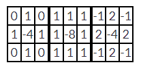
模板实际上是根据离散数据求近似二阶导数的公式，整理得到的矩阵形式。

2.LoG算子

由于Laplacian算子对噪点敏感，常常在Laplacian处理前对图片进行高斯滤波，为了简化运算，将高斯滤波算子与Laplacian算子相结合，就得到了LoG算子:



而当高斯滤波范围很窄（方差很小）时，高斯滤波不再产生影响，LoG算子退化为Laplacian算子。

3.编程实现

参考网站的代码有一个严重的错误

第27行的image应改为new_image，以将new_image的灰度值缩放到0~255范围内。
下面是更正后的代码

# LoG边缘检测算子
def LaplaceOperator(roi, operator_type="fourfields"):
    if operator_type == "fourfields":
        laplace_operator = np.array([[0, 1, 0], [1, -4, 1], [0, 1, 0]])
    elif operator_type == "eightfields":
        laplace_operator = np.array([[1, 1, 1], [1, -8, 1], [1, 1, 1]])
    else:
        raise ("type Error")
    result = np.abs(np.sum(roi * laplace_operator))
    return result


def LaplaceAlogrithm(image, operator_type="fourfields"):
    # 提取结果
    new_image = np.zeros(image.shape)
    # 扩充边界
    image = cv2.copyMakeBorder(image, 1, 1, 1, 1, cv2.BORDER_DEFAULT)
    for i in range(1, image.shape[0] - 1):
        for j in range(1, image.shape[1] - 1):
            new_image[i - 1, j - 1] = LaplaceOperator2(image[i - 1:i + 2, j - 1:j + 2], operator_type)
    # 归一
    new_image = new_image * (255 / np.max(new_image))
    return new_image.astype(np.uint8)

4.与OpenCV官方函数的比较

下面比较了OpenCV与自编写函数的边缘提取效果，处理图像为经典的Lena图：

代码如下：

def main():
    for image_path in settings.IMAGE_PATHS:
        # 读取图片
        image = cv2.imread(image_path)
        image = cv2.cvtColor(image, cv2.COLOR_RGB2GRAY)
        # image = cv2.GaussianBlur(image, (3, 3), 0.000001)
        # 官方提取结果
        log_image0 = cv2.Laplacian(image, -1, ksize=1)
        # 自编写函数提取结果
        log_image1 = LaplaceAlogrithm(image, "fourfields")
        # 做差比较
        diff_image = utils.minus_image(log_image0, log_image1)
        # 保存结果
        results = [log_image0, log_image1, diff_image]
        labels = ['cv', 'mine', 'diff']
        name = utils.get_filename(image_path)
        for result, label in zip(results, labels):
            path = os.path.join(OUTPUT_PATH, name + '-' + label + '.bmp')
            utils.save_image(result, path)

结果如下：
OpenCV处理结果

自编写函数处理结果

图片做差结果

可见自编写函数的边缘提取效果不如官方函数。
根据cv2.Laplacian函数申明：

当ksize参数设为1时，确实使用Laplacian算子的第一个模板进行处理，与自编写的函数的处理相同，但结果却存在较大差异，原因可能是OpenCV的优化比较好。

二、Canny算子

1.概述

Canny算子是John.F.Canny于1986年提出的边缘提取算子，现被广泛应用于计算机视觉领域，传统的Canny边缘提取算法主要包含如下五个步骤：
1.高斯滤波，抑制噪声
2.求梯度阵
3.非极大抑制，保证边缘点的准确性
4.双阈值检测，抑制噪声产生的假边缘
5.中值边缘点的筛选

2.代码实现

参考：https://www.jianshu.com/p/effb2371ea12
我在上述代码的基础上做了许多更正与优化，修改后代码如下：

def NMS0(d, dx, dy):
    W2, H2 = d.shape
    NMS = np.copy(d)
    NMS[0, :] = NMS[W2 - 1, :] = NMS[:, 0] = NMS[:, H2 - 1] = 0
    for i in range(1, W2 - 1):
        for j in range(1, H2 - 1):
            # 如果当前梯度为0，该点就不是边缘点
            if d[i, j] == 0:
                NMS[i, j] = 0
            else:
                gradX = dx[i, j]
                gradY = dy[i, j]
                gradTemp = d[i, j]

                # 如果Y方向幅度值较大
                if np.abs(gradY) > np.abs(gradX):
                    weight = np.abs(gradX) / np.abs(gradY)
                    grad2 = d[i - 1, j]
                    grad4 = d[i + 1, j]
                    # 如果x,y方向梯度符号相同
                    if gradX * gradY > 0:
                        grad1 = d[i - 1, j - 1]
                        grad3 = d[i + 1, j + 1]
                    # 如果x,y方向梯度符号相反
                    else:
                        grad1 = d[i - 1, j + 1]
                        grad3 = d[i + 1, j - 1]

                # 如果X方向幅度值较大
                else:
                    weight = np.abs(gradY) / np.abs(gradX)
                    grad2 = d[i, j - 1]
                    grad4 = d[i, j + 1]
                    # 如果x,y方向梯度符号相同
                    if gradX * gradY > 0:
                        grad1 = d[i + 1, j - 1]
                        grad3 = d[i - 1, j + 1]
                    # 如果x,y方向梯度符号相反
                    else:
                        grad1 = d[i - 1, j - 1]
                        grad3 = d[i + 1, j + 1]

                gradTemp1 = weight * grad1 + (1 - weight) * grad2
                gradTemp2 = weight * grad3 + (1 - weight) * grad4
                if gradTemp >= gradTemp1 and gradTemp >= gradTemp2:
                    NMS[i, j] = gradTemp
                else:
                    NMS[i, j] = 0
    return NMS


def NMS1(d, dx, dy):
    theta0 = [0, 180, -180]
    theta45 = [45, -135, 225]
    theta90 = [90, -90, 270, -270]
    theta135 = [-45, 135, -225]
    # 梯度方向矩阵,单位转换为°
    NMS = np.zeros(d.shape)
    theta = np.arctan2(dy, dx) / np.pi * 180
    # 梯度取整
    theta = np.round(theta / 45) * 45
    for r in range(1, d.shape[0] - 1):
        for c in range(1, d.shape[1] - 1):
            current_theta = theta[r][c]
            if d[r][c] == 0:
                continue
            if current_theta in theta0:
                if d[r][c] >= d[r][c + 1] and d[r][c] >= d[r][c - 1]:
                    NMS[r][c] = d[r][c]
            if current_theta in theta45:
                if d[r][c] >= d[r + 1][c - 1] and d[r][c] >= d[r - 1][c + 1]:
                    NMS[r][c] = d[r][c]
            if current_theta in theta90:
                if d[r][c] >= d[r + 1][c] and d[r][c] >= d[r - 1][c]:
                    NMS[r][c] = d[r][c]
            if current_theta in theta135:
                if d[r][c] >= d[r - 1][c - 1] and d[r][c] >= d[r + 1][c + 1]:
                    NMS[r][c] = d[r][c]
    NMS = NMS * 255 / np.max(NMS)
    return NMS


def run(image, th1, th2):
    if th1 > th2:
        temp = th1
        th1 = th2
        th2 = temp
    # step1.高斯滤波
    #image = cv2.GaussianBlur(image, (3, 3), 0.5)
    # step2.增强 通过求梯度幅值
    # W1, H1 = image.shape
    # dx = np.zeros([W1 - 1, H1 - 1])
    # dy = np.zeros([W1 - 1, H1 - 1])
    # d = np.zeros([W1 - 1, H1 - 1])
    # for i in range(W1 - 1):
    #     for j in range(H1 - 1):
    #         dx[i, j] = image[i, j + 1] - image[i, j]
    #         dy[i, j] = image[i + 1, j] - image[i, j]
    #         d[i, j] = np.sqrt(np.square(dx[i, j]) + np.square(dy[i, j]))  # 图像梯度幅值作为图像强度值
    dx = cv2.Sobel(image, cv2.CV_16S, 1, 0).astype(np.float)
    dy = cv2.Sobel(image, cv2.CV_16S, 0, 1).astype(np.float)
    d = np.sqrt(dx * dx + dy * dy)
    # setp3.非极大值抑制 NMS
    NMS = NMS1(d, dx, dy)
    # step4. 双阈值算法检测、连接边缘
    W3, H3 = NMS.shape
    DT = np.zeros([W3, H3])
    # 定义高低阈值
    TL = th1 * np.max(NMS)
    TH = th2 * np.max(NMS)
    ca = 2
    for i in range(1, W3 - 1):
        for j in range(1, H3 - 1):
            if (NMS[i, j] < TL):
                DT[i, j] = 0
            elif (NMS[i, j] > TH):
                DT[i, j] = 255
            elif ((NMS[i - ca:i + ca, j - ca:j + ca] > TH).any()):
                DT[i, j] = 255
    return DT

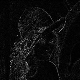
3.与OpenCV官方函数的比较

OpenCV结果：
自编写函数结果：
两图片差值：

从Lena的眼部与头发部分可以看出，OpeCV的提取结果更好，边缘更加真实，主要原因是因为我们实现的是传统的Canny算法，如今的Canny算法在此基础之上做了许多优化，可参考Wiki的Canny算子的优化。