Lecture 5——DNA-seq-2_Bioinformatics and Statistical Topics
本文图片来自于学习视频——新一代测序技术数据分析第五讲 DNA-seq2_Bioinformatics and Statistical Topics
Sequence mappability
Human genome
The minimum length (number of nucleotides) can be uniquely mapped back to human genome?
In theory, reads with 16 bases or more can be uniquely mapped back to human genome
~half of human genome is repetitive DNA
Available for download at UCSC Genome Browser, display how uniquely k-mer sequences align to a region of the genome (k=24, 36, 40, 50, 75, and 100)
S= l/(number of matches found in the genome), 2 mismatches allowed; i.e. S= 1(unique)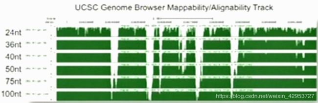
Generate your own mappability track
Mappability is determined by multiple factors
the alignment algorithm (Koehler et al. Bioinformatics, 2010)
the regions where mapping occur
the biochemistry assay
Regions can be slightly different
Refined alignment
Sequence alignment
Number of mismatching bases minimized across one read
Sequence refined alignment
Number of mismatching bases minimized across all the reads
What went wrong for the initial alignment?
A large percent of regions requiring local realignment are due to the presence of an insertion or deletion (indels) in the individual’s genome with respect to the reference genome
The aligner prefers one/two mismatches over a 4bp insertion
Such alignment artifacts result in many bases mismatching the reference near the misalignment, which are mistaken as SNPs
Initial mapping treats each read independently
Even when some of the reads are correctly mapped with indels, reads covering the indels near just the start and end are often misaligned.
Local realignment
Transform regions with misalignments due to indels into clean reads containing a consensus indel suitable for standard variant discovery approaches.
Two steps
1: Determining (small) suspicious intervals which are likely in need of realignment
2: Running the realigner over those intervals
Step 1
De novo indels in initial alignment
If one or more reads contain an indel (and are aligned correctly). one would want to make sure that the indel containing reads in the pileup are aligned correctly
No indels identified in the initial alignment
with base call: clustered SNP calls, which is suspicious and are often caused by indels
Without base call: detect clustered loci with high entropy ( i.e. lots of mismatches)
For known indels in dbSNP
Step 2
Construct all possible haplotypes by integrating
Reference genome
Known gaps
De novo gaps (by BFAST/BWA, or Smith-Waterman)
Conduct gapless alignment against all possible haplotypes, and calculate the likelihood of each haplotype
Key information on realignment
Minimizing mismatches for one read vs. multiple reads
Realignment process:
Enumerate potential haplotype candidates
Conduct gapless alignment on all haplotypes
Calculate likelihood for each haplotype
USE WITH CAUTION
Major assumption: consistency in the inferred haplotypes among all individuals
Doesn’t work on somatic SNP and indel alling (semi-random process)
Needs to have significant improvement to replace the initial alignment. May not work for:
pool seq experiment if only a small portion of individual has the indel
RNA-seq experiment if the low expressed allele contains the indel
Quality and recalibration
available covariates
Cycle Covariate(machine cycle for this biase), DinucCovariate, HomopolymerCovariate, MappingQualityCovariate, Minimum NQSCovariate, PositionCovariate, PrimerRoundCovariate, QualityScoreCovariate, ReadGroupCovariate
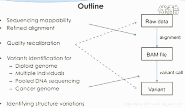
Variant identification
Diploid genome, Multiple individuals, Cancer genome/pooled sequencing
So, It is not that straightforward
Sequencing error should be considered
How to call a variant
Factors to be considered
Number of reads supporting each genotype(10G/1A vs. 5G/6A)
Base quality for each nucleotide
Alignment quality for each read
Sequence depth
Sequencing error —— machine related
Output: probability for each genotype(AA, A/G, or GG)
Bayesian approach
Bayesian inference is a method of statistical inference in which evidence is used to update the uncertainty of parameters and predictions in a probability model
One locus, n reads
k reads support A
n-k reads support G
Three possible genotypes
: observing n-k errors (G) in n reads
: binomial mode. In theory, we should have half A reads, and half G reads
: observing k errors (A) in n reads
Variant Quality
Prior of genotypes:
P = P = (1-r)/2
P = r
r is pre-defined probability of observing heterozygotes
r = 0.2 for known SNP loci
r = 0.001 for unknown loci
Posterior probability of p(g | D)
p(g | D) = p(g)* p(D|G)/P(D)
P(D) = p(D|)P()+p(D|)p()+p(D|)p()
Variant quality:
Q = -10log10(1-p(g| D))
Additional comments
This method only works for diploid genome
Require substantial coverage for each genomic loci (>20x coverage)
This is not always the case
For low to moderate sequence coverage, this won’t work
Lead to under-calling heterozygous
One assumption: independence among reads
Genotype based on multiple individuals
Variant calls based on multiple individuals dramatically increased the accuracy
Neilsen et al. Nature Reviews Genetics, 2010
Somatic variants/pooled sequencing
Different interpretation
Dipoid genome: homozygote. A is a sequencing error
Somatic seq: a novel mutation
Pooled sequencing: a rare variant
RNA-seq: G allele express much more than A allele
Assumption
2 possible nucleotides, the third most abundant is “error”
Several published approaches
SNPSeeker —— based on large deviation theory(Druley et a., Nature Methods, 2009)
SNVMix2 —— a probabilistic Binormial mixture model (Goya et al. Bioinformatics, 2010)
SNVer—— a binomial-binomial model( Wei et al., NAR, 2011)
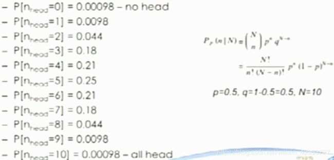
Binomial distribution
Toss coins —— probability getting a head or tail is 50%
Variant quality recalibration
Machine/Chemistry artifacts
Sequencing cycles, different chemistry versions, GC-rich regions are hard to sequence, homopolymers, sequence bias…
Analysis flaws
Systematic alignment inaccuracy, …
Each variant has many variables
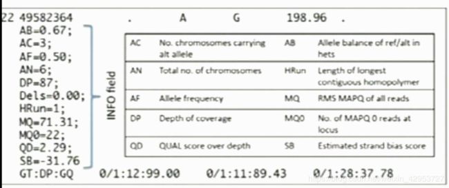
Variation quality
Depth of coverage
Strand bias
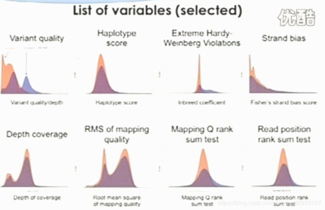
Most of the info is in the VCF file
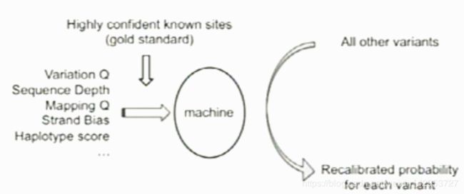
Recalibraiton strategy
Training on highly confident known sites to determine the probability that other sites are true.
Machine learning strategy
Gold standard
Annotated variants: Identified variants already present in HapMap3, which includes 1301 samples.
Model:
Variational Bayes Guassian mixture model
Evaluation for the SNP call quality
Expected number of calls
The number of SNP calls should be close to the average human heterozygosity of 1 variant per 1000 bases.
Concordance with genotype chip calls
What fraction of SNPs are already known
dbSNP catalogs most common variation, so most of the true variants found will be in dbSNP
For single sample calls, ~90% of variants should be in dbSNP
Need to adjust expectation when considering calls across samples.
Transition to transversion ration(Ti/Tv)
Transitions are twice as frequent as transversions
Validated human SNP data suggests that the Ti/Tv should be ~2.1 genome-wide and ~2.8 in exons
sFP SNPs should has Ti/Tv around 0.5
Ti/Tv is a good metric for assessing SNP call quality
Structural variations
insertions or inversions > 1kb
Often involves repetitive regions of the genome and complex rearrangements
No optimal method for SV discovery
Analysis of the 1000 Genome Project pilot data identified a total of 1775 SVs that affect coding sequence.
Methods based on tag density
Methods using depth of coverage
Genome is divided into multiple non-overlapping windows
Count the number of reads fell in each window
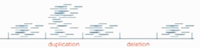
Assumption: sequencing reads are randomly sampledwith equal probability from any location on the sequenced genome. After aligning these reads to the reference genome, the read density of a given genome window should be proportional to the local copy number.
Density is also determined by other factors including GC content, mappability,…
Yoon et al., Bailey et al., Volik et al., Cambell et al., Alkan et al.
Case-control design
Look for the genomic regions with contains significantly more (or fewer) case reads than the control reads.
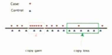
Assumption: bias for case and control genomes are similar
Application: Comparing tumor genome versus matched normal genome
Strategy
Partition the genome into fixed window size
Compare tag density in each window
Correct for multiple testing
Choice for window size is tricky and important
Too big decreased resolution
Too small decreased power ( more windows, more test)
Solution
Optimize the window size given a significance level. Xie and Tammin, BMC Bioinformatics, 2009)——window merging is required
Focused on the identification of breakpoints rather than CNV regions(SegSeq, Chiang et al, Nature Methods. 2009)——improved power to identify small but significant regions
Methods using paired-end mapping (PEM)
look for discordant PEMs that may indicate the presence of SVs nearby
Xi et al., Brief. Fun Genomics 2011
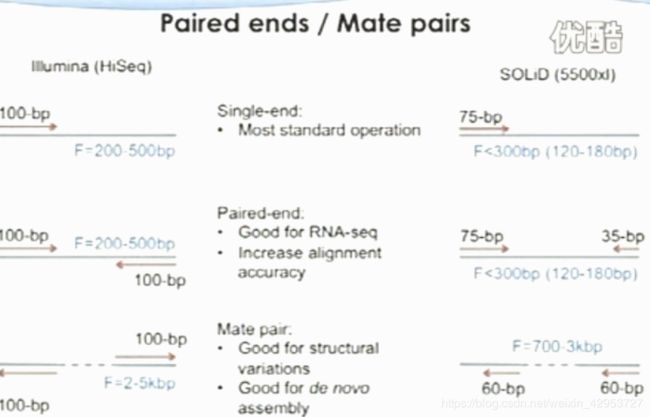
Paired ends/ Mate pairs
Cluster-based methods
Tuzun et al. Korbel et al.
only for large SVs
Distribution-based methods
Compare the local distribution of thw mapped distances to the genome wide distribution of insert sizes.
Chen et al. Nat Method 2009