Byte Tank
Deep Reinforcement Learning: Playing a Racing Game
Agent playing Out Run, session 201609171218_175eps
No time limit, no traffic, 2X time lapse
Above is the built deep Q-network (DQN) agent playing Out Run, trained for a total of 1.8 million frames on a Amazon Web Services g2.2xlarge (GPU enabled) instance. The agent was built using python and tensorflow. The Out Run game emulator is a modified version of Cannonball. All source code for this project is available on GitHub.
The agent learnt how to play by being rewarded for high speeds and penalized for crashing or going off road. It fetched the game’s screens, car speed, number of off-road wheels and collision state from the emulator and issued actions to it such as pressing the left, right, accelerate or brake virtual button.
Agent trainer implements the deep Q-learning algorithm used by Google’s DeepMind Team to play various Atari 2600 games. It uses a reward function and hyperparameters that fit best for Out Run, but could potentially be used to play other games or solve other problems.
There is a wealth of good information about this reinforcement learning algorithm, but I found some topics difficult to grasp or contextualize solely from the information available online. I will attempt to add my humble contribution by tackling these and also provide details about the project’s implementation, results and how it can be used/modified/deployed.
Let’s start by one of its main gears: Q-learning
Concepts
Q-learning
At the heart of deep Q-learning lies Q-learning, a popular and effective model-free algorithm for learning from delayed reinforcement.
Jacob Schrum has made available a terse and accessible explanation which takes around 45 minutes to watch and serves as a great starting point for the paragraphs below. Let’s take the canonical reinforcement learning example presented by Jacob (grid world):
To implement this algorithm, we need to build the Q-function (one of the forms of the Bell-Equation) by using the Q-value iteration update:
In the above grid, there are 9 actionable states, 2 terminal states and 4 possible actions (left, right, up, down), resulting in 36 (9 actionable states x 4 possible actions) Q-values.
This project aims to train an agent to play Out Run via its game screens, so for the sake of argument, let´s consider that each game screen is transformed into a 80x80 greyscale image (each pixel value ranging from 0 to 255), and that each transformed image represents a state. 6400 pixels (80x80) and 256 possible values per pixel translate to 2566400 possible states. This value alone is a good indicator of how inflated the number of possible Q-values will be.
Multiplying 9 possible actions by 2566400 possible states results in 2566400 x 9 possible Q-values. If we use multiple and/or colored images for state representation, then this value will be even higher. Quite unwieldy if we want to store these values in a table or similar structure.
Enter neural networks
Artificial neural networks work quite well for inferring the mapping implied by data, giving them the ability to predict an approximated output from an input that they never saw before. No longer do we need to store all state/action pair’s q-values, we can now model these mappings in a more general, less redundant way.
This is perfect. We can now use a neural network to model the Q-function: the network would accept a state/action combination as input and would output the corresponding Q-value. Training-wise, we can feed in the state/action combo to get the network’s Q-value output, and calculate the expected Q-value using the formula above. With these two values, we can perform a gradient step on the (for example) squared difference between the expected value and the network’s output.
This is perfect, but there is still room for improvement. Imagine we have 5 possible actions for any given state: to get the optimal future value estimate (consequent state’s maximum Q-value) we need to ask (forward pass) our neural network for a Q-value 5 times per learning step.
Another approach (used in DeepMind’s network) would be to feed in the game’s screens and have the network output the Q-value for each possible action. This way, a single forward pass would output all the Q-values for a given state, translating to one forward pass per optimal future value estimate.
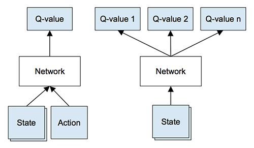
Q-learning and neural networks are the center pieces of a deep Q-network reinforcement learning agent and I think that by understanding them and how they fit together, it can be easier to picture how the algorithm works as a whole.
Implementation
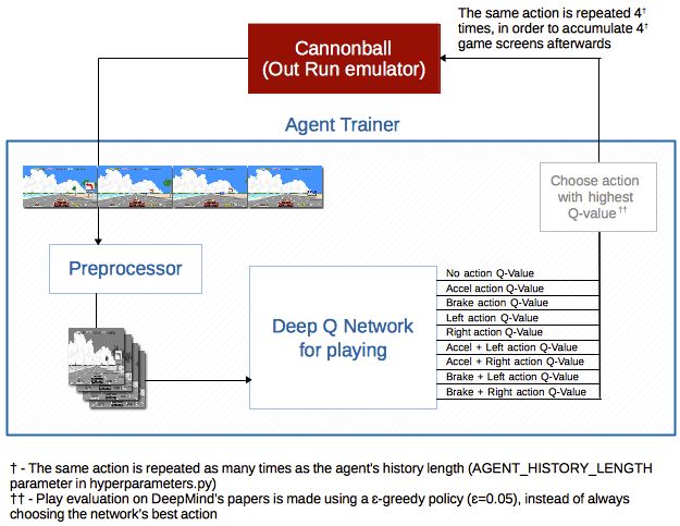
Above is an overall representation of how the different components relate during a play evaluation, centered around the deep Q-network for playing1, the main decision component.
Each game screen is resized to a desaturated 80x80 pixels image (opposed to 84x84 on DeepMind’s papers), and if you might be wondering why each state is a sequence of four game screens instead of one, that is because the agent’s history is used for better motion perception. Achieving this requires a sequence of preprocessed images to be stacked in channels (like you would stack RGB channels on a colored image) and fed to the network. Note that RGB channels and agent history could be used simultaneously for state representation. For example, with three channels per (RGB) image and an agent history length of four, the network would be fed twelve channels per input state.
The network’s architecture is essentially the same used by DeepMind, except for the first convolutional neural network’s input (80x80x4 instead of 84x84x4, to account for the different input sizes) and the linear layer’s output (9 instead of 18, to account for the different number of actions available)
The algorithm used to train this network is well described here (page 7) and here, but I would like to present it graphically, to hopefully provide some further intuition.
Below is agent trainer´s implementation of the aforementioned algorithm. It adds some new concepts which were not approached by this article:
- Experience replay mechanism sported by replay memories: randomly samples previous transitions, thereby smoothing the training distribution over many past behaviors
- Separate training network, cloned at fixed intervals to the target playing network, making the algorithm more stable when compared with standard online Q-learning
- ε-greedy policy to balance exploitation/exploration

Reward function
The reward function’s definition is crucial for good learning performance and determines the goal in a reinforcement learning problem. April Yu et al. have an interesting paper on simulated autonomous vehicle control which details a DQN agent used to drive a game that strongly resembles Out Run (JavaScript Racer). Based on their reward function experiments, I’ve built a function which rewards logarithmically based on speed and penalizes when the car is off-road, crashed or stopped.

Deployment
Run the trainer and emulator on your local machine by following the guide available on agent-trainer’s readme.
It is also possible to deploy the agent to an AWS EC2 instance or generic Linux remote machine by using a set of bash scripts offered by agent-trainer-deployer.
AWS EC2
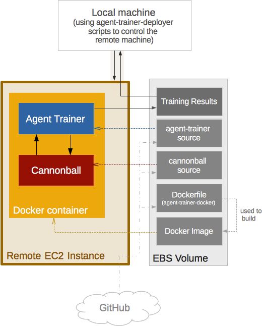
Amazon allows you to bid on spare EC2 computing capacity via spot instances. These can cost a fraction of on-demand ones, and for this reason were chosen as the prime method for training in this project, leading to the need for mid-training instance termination resilience.
To accommodate this scenario, the deployment scripts and agent-trainer are designed to support train session resumes. To persist results and decrease boot up time between sessions, a long-lived EBS volume is attached to the live instance. The volume contains the training results, agent-trainer´s source code, cannonball’s source code, dockerfiles and their respective docker images.
Results
The hyperparameters used on all sessions mimic the ones used on DeepMind’s Human-Level Control through Deep Reinforcement Learning paper, except for the number of frames skipped between actions, which are spaced apart by 450ms (equivalent to 13 frames) on agent-trainer.
The Out Run game, as you would play it in an arcade, clutters the road with various cars in order to make the game more challenging. In-game traffic was disabled for both training and evaluation plays, rendering a more achievable starting point for these experiments. Training with random traffic could be an interesting posterior experiment.
Some experiments were made by increasing the discount factor up its final value during training, as proposed on “How to Discount Deep Reinforcement Learning: Towards New Dynamic Strategies”, but did not achieve better stability or rewards when compared to a fixed 0.99 discount factor. The aforementioned paper also proposes decaying the learning rate during training, which increased stability and performance significantly. Decaying the learning rate without minimum value clipping yielded the best results.
Another improvement was to train the game without a time limit, meaning that the training episode would only finish when the car reached the last stage’s end. This allowed for a broader replay memory training set, since the agent traversed a wide range of different tracks and settings.
Play evaluation was the same between all experiments, this is, the agent was evaluated by playing on the default 80 second, easy mode.
Here is a summary of the most relevant training sessions (you can find their models, metrics and visualizations on agent-trainer-results):
| Session | M | Training game mode |
Learning rate decay |
|---|---|---|---|
| 201609040550_5010eps | a) | timed; easy | without learning rate decay |
| 201609111241_2700eps | b) | timed; easy | unclipped learning rate decay |
| 201609111241_7300eps | b) | timed; easy | unclipped learning rate decay |
| 201609160922_54eps | b) | unlimited time | without learning rate decay |
| 201609171218_175eps | b) | unlimited time | unclipped learning rate decay |
Training sessions summary: session names are formed by
(M)achine used: a) AMD Athlon(tm) II X2 250 Processor @ 3GHz; 2GB RAM DDR3-1333 SDRAM; SSD 500 GB: Samsung 850 EVO (CPU only training); b) AWS EC2 g2.2xlarge (GPU enabled instance), 200 GB General Purpose SSD (GP2)
Agent playing Out Run (timed easy mode, no traffic)
Session 201609111241_2700eps
Agent playing Out Run (timed easy mode, no traffic)
Session 201609171218_175eps
Notice on the videos above how the timed mode trained session 201609111241_2700eps reaches the first checkpoint about five seconds earlier than the unlimited time mode trained session 201609171218_175eps, but proceeds to drive off-road two turns after. Its stability gets increasingly compromised as more episodes are trained, which can be observed by the rampant loss increase before 7300 episodes are reached (201609111241_7300eps):


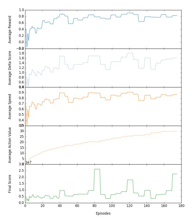
Both 201609111241_2700eps and 201609111241_7300eps timed trained sessions mostly drive off-road and stall after the first stage, whereas the unlimited time mode trained session 201609171218_175eps can race through all the stages crashing only three times (as shown on the article’s first video) and is able to match the performance of a timed trained session when evaluated on the default easy timed mode.
Below is the loss plot for 201609160922_54eps and 201609171218_175eps, both trained using the game’s unlimited time mode, difference being that 201609160922_54eps keeps a fixed learning rate and 201609171218_175eps decays it every 50100 steps:

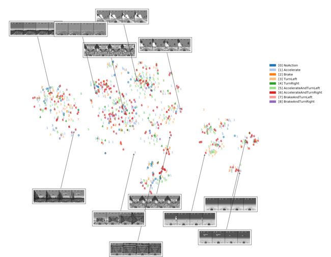
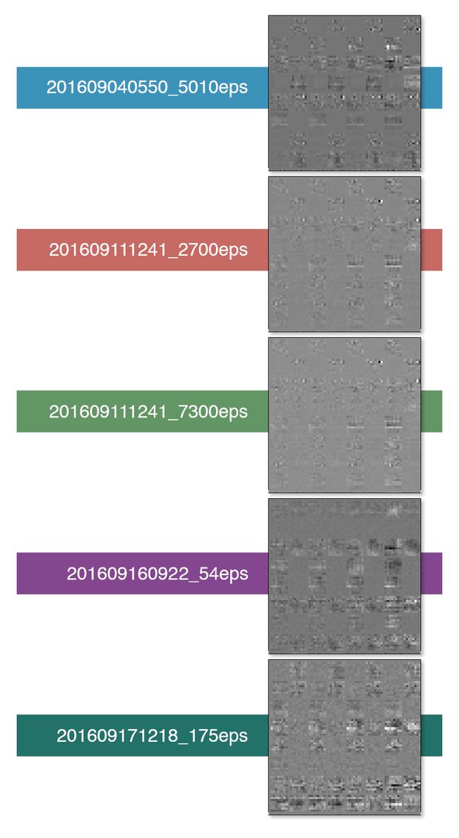
Other representative visualizations:

Final Notes
Plugging other problems and games
Agent-trainer was not built from the get-go to train games or problems other than Out Run, but I think it would be interesting to perform a thought exercise on what would be necessary to do so.
There are three main areas in which agent-trainer has domain knowledge about Out Run:
gamepackage, which containsActionenumeration: describes all the possible actions in the game.cannonball_wrappermodule: only this module has access to the cannonball emulator. It translates the aforementioned actions into game actions and is accessed by methods such asstart_game(),reset()andspeed().
RewardCalculatorclass: contains the reward function. Instead of using a generic reward function like DeepMind, it was chosen to have a tailor-made reward function for Out Run, which takes into account the car’s speed and its off-road and crash status.metricsmodule: aware of thespeedmetric, which is Out Run specific, andscore, which is game specific domain knowledge.
Training another game would require the creation of a new wrapper with the same interface as cannonball_wrapper, a new Action enumerator specific to the game, a new RewardCalculatorwith a different reward function and the removal/replacement of the speed metric.
Apart from the previously mentioned steps, solving generic problems would require the preprocessor to be changed/replaced if images were not to be used for state representation. An option would be to create a new preprocessor class with a process(input) method, tweak the hyperparameters as required (so that the network knows which dimensions to expect on its input), and finally inject the newly created class in EpisodeRunner, replacing the old preprocessor class.
Further references
I am not a machine learning expert, but from my learner’s point of view, if you are interested in getting your feet wet, Andrew Ng’s Machine Learning Course is as a great starting point. It is freely available on the Coursera online learning platform. This was my first solid contact with the subject and served as a major stepping stone for related topics such as Reinforcement Learning.
Udacity Google Deep Learning: this free course tackles some of the popular deep learning techniques, all the while using tensorflow. I did this right after Andrew Ng’s course and found it to leave the student with less support during lessons - less hand-holding if you will - and as result I spent a good amount of time dabbling to reach a solution for the assignments.
As a side note, I started building this project by the end of the Deep Learning course, mostly because I wanted to apply and consolidate the concepts I learnt into something more practical and to share this knowledge further, so it could hopefully help more people who are interested in this.
Other useful resources:
- DeepMind’s Human-Level Control through Deep Reinforcement Learning paper and its respective source code
- Playing Atari with Deep Reinforcement Learning
- Deep Reinforcement Learning for Simulated Autonomous Vehicle Control
- Demystifying Deep Reinforcement Learning
- Udacity Reinforcement Learning by Georgia Tech
- Deep learning lecture by Nando de Freitas
- Learning reinforcement learning (with code, exercises and solutions)
- OpenAI Gym: quoting the project’s page: ”a toolkit for developing and comparing reinforcement learning algorithms. It supports teaching agents everything from walking to playing games like Pong or Go”
- Tensorflow implementation of Human-Level Control through Deep Reinforcement Learning, by Devsisters corp.
Source code
All source code is available on GitHub:
- Agent Trainer: the core python+tensorflow application
- Cannonball: custom Cannonball (Out Run game emulator) fork which contains the changes needed to access the emulator externally
- Agent Trainer Deployer: bash scripts to deploy agent-trainer to a generic remote machine or AWS EC2 instance
- Agent Trainer Docker: Dockerfiles used when deploying agent-trainer to a remote machine
- Agent Trainer Results: Collection of training sessions, each containing their resulting network, metrics and visualizations
-
“Deep Q-network for playing” in this project is equivalent to DeepMind’s “target network Q^Q^” and “Deep Q-network for training” is equivalent to DeepMind’s “network Q”↩
Comments
Copyright © 2016 - Pedro Lopes - Powered by Octopress. Theme based on Whitespace. Subscribe via RSS Feed
