大三的统计计算大作业

Control variate estimation using estimated control means

student name	Student ID	Course	instructor
Luo Cheng	07317120	statistical calculation	Xu Liang

Abstract: The question of interest in the article is whether the true value \(\mu_y\) in the control variable method \(Z=X+c^*(Y-\mu_y)\) can be replaced by its estimate, i.e. \(Z_{cv}=X+c'(Y-\hat\mu_y)\),and the relationship between the two different method.

Contents

1、 Question posed

1.1 Question: Using estimates for the mean \(\mu_y\)

The traditional algorithm of the control variable method requires that the mean of the control variable \(E[Y]=\mu_y\) is known and that \(Z=X+c(Y-\mu_y)\) is an unbiased estimate of \(\theta\); the variance is

\[VarZ=Var(X+cY)\\=Var(X)+c^2Var(Y)+2*cCov(XY) \]

At this point, from the knowledge of first-order derivatives, it is known that

\[\frac{\partial Var(Z)}{\partial c}=0 \Rightarrow c^*=-\frac{Cov(X,Y)}{Var(X)}. \]

At this point we get the variance \(Var(Z) = Var(X)-\frac{Cov(X,Y)^2}{Var(Y)}\), where the reduced amount of variance

\[\frac{Var(X+c^*(Y-\mu_y))}{Var(X)}=1-Corr^2(X,Y) \]

, where \(Corr(X,Y)=\rho=\frac{Cov(X,Y)}{\sqrt{Var(X)Var(Y)}}\) represents the correlation coefficient of \(X,Y\).

But when we don't know the true value of \(\mu_y\), can we use the control variable method, that is, \(\mu_y\) in \(Z=X+c(Y-\mu_y)\) using the estimated amount \(\hat{\mu_y}\)? What are the gaps and links between this and traditional control variables?

1.2 literature review

​ The control variables method is a widely used variance reduction method, the basic principle of which is "use what you know". Foreign scholars have studied it extensively, Lavenher and Welsh use control variables. Achieving estimates of univariate means, Glynn gives a study of the asymptotic efficiency of parameters in variance reduction, Schmeiser takes into account the biased mean values of the control variables, Pasupathy at The control variables are biased on the basis of their mean values, giving unbiased estimates of the mean values, Yang applies the idea of the dipole variable to the control variables, etc. There are relatively few domestic studies, Zhengjun Zhang et al. give a review of variance reduction methods in stochastic system simulation.

2、 theoretical research

2.1 The mean estimates of the control variables are unbiased estimates

We know at this point that its estimated estimate is an unbiased estimate, at which point we can first estimate the mean of the control variable \(\hat\mu_y\) with an additional sample. Re-use the estimate to quantify \(\hat{\mu_y}\) instead of \(\mu_y\) in the conventional estimate, where \(\hat{\mu_y}\thicksim AN(\mu_y,\frac{Var(Y)}{k'})\), where \(k'\) is the sample size when the mean of the control variable is estimated. This error

\[\varepsilon=\hat{\mu_y}-\mu_y\thicksim AN(0,\frac{Var(Y)}{k'}). \]

On a sub-basis, we construct new mean-estimate-based expressions:

\[Z=X+c(Y-\hat{\mu_y}) \]

We use auxiliary experiments to estimate, introducing a new error, which is a biased estimate, and we will discuss the minimization of the mean square error.

2.2 \(MSE\) variance reduction

For general,

\[MSE(\hat{\theta})=Var(\hat{\theta})+(E(\hat{\theta})-\theta)^2 \]

, but at this point we do not know the true case of the deviation of each fit, but we already know that the expectation of the deviation is \(E[(c\varepsilon)^2]=\frac{c^2Var(Y)}{k'}\).

To obtain the smallest case of \(MSE\),

\[MSE(Z,\theta|\varepsilon)=E_{y}[Var[Z|\varepsilon]]+(E(Z)-\theta)^2\\=\frac{Var(X)}{k}+c^2\times\frac{Var[Y]}{k}+2c\frac{Cov(X,Y)}{k}+E_y[(c\varepsilon)^2]\\ =\frac{Var(X)}{k}+c^2\times\frac{Var[Y]}{k}+2c\frac{Cov(X,Y)}{k}+c^2\frac{Var(Y)}{k'} \]

Setting the first derivative of \(MSE[Z,\theta]\) to zero yields the \(MSE\)-optimal control-variate weight:

\[\frac{\partial MSE}{\partial c}=0\Rightarrow c(k')=-\frac{Cov(X,Y)}{Var(Y)}(\frac{1}{1+\frac{k}{k'}}) \]

substituting \(c(k')\) into the upper equation, we get the mean error of

\[MSE[Z_{cv}(c(k')),\theta]=MSE[\bar{\mu_x},X]\times[1-\rho^2(\frac{1}{1+\frac{k}{k'}})]. \]

Obviously the variance is reduced, and the reduced brightness of the variance is \(\rho^2(\frac{1}{1+\frac{k}{k'}})\), where \(\rho\) is \(Corr(X,Y)\).

If \(k' = 0\), then \(c(k') = 0\) and the direct-simulation experiment is optimal. The \(MSE\)-optimal auxiliary sample size is \(k' = \infty\), in which case \(c(k')\) and \(MSE[Z_{cv}(c(k')),\theta]\) correspond to the classical values .

2.3 \(k'\)Discussion of extreme values

We look at the analysis of the results in two extreme cases:

• \(k'=0\)

When $c(k')=0\Rightarrow $ this straightforward no-use variance reduction technique.

• \(\lim k' \rightarrow +\infty\)

When \(k'=\infty\) is equal to the effect of knowing the true value of \(\mu_y\).

So we can get that when \(k'\) varies between \(0\thicksim \infty\), the variance of the variance is not between using the control variable and using the control variable.

3. Simulation examples

3.1 Examples-1

Compute \(E[e^x]\) where \(X \thicksim N(\mu,\sigma)\) and the control variable chosen is \(X \thicksim N(\mu,\sigma)\)

3.1.1 Code and results presentation

The simulation can be continued with the \(k'\) continuing to increase, and results such as theoretical analysis can be obtained. At \(k'\rightarrow \infty\) is the tendency to know the true worthiness of \(\mu_y\), i.e. the traditional control variable method.

Below we demonstrate the convergence process using the visualization results.

3.1.2 Visualization of the convergence process

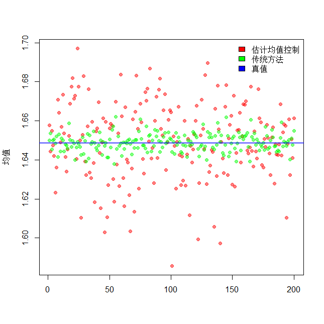
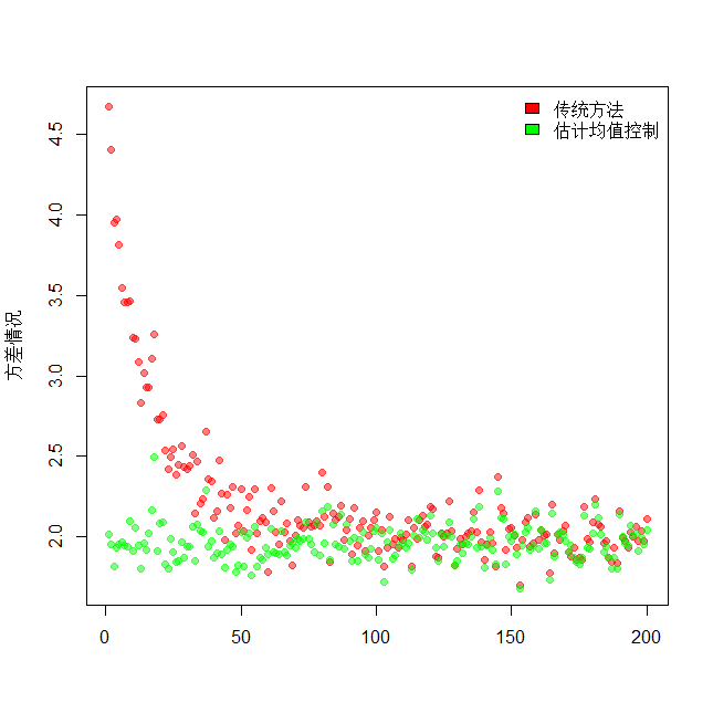
Code display, adding loops makes \(k'\rightarrow\infty\).We actually got good results when \(k'\) was 5000.

rm(list = ls())

#初始化数据
MinNum = 10;MaxNum = 10000;
ExpectNum = seq(MinNum,MaxNum,by = 50)#用于设置k'的值变化
PilotNum = 1000
MainNum = 100000
#储存数据的集合
n=length(ExpectNum)
MeanHandEx = c(NA)
MeanHandExByEx = c(NA)
VarHandEx = c(NA)
VarHandExByEx = c(NA)

i=1 #index
for (HBEi in ExpectNum) {
  
  # /*Do pilot simulation first*/
  RepCData <- rnorm(PilotNum)
  conditionYC <-RepCData 
  xc <- exp(RepCData)
  RegModel <- lm(xc~conditionYC)
  StarC <- -RegModel$coefficients[2]
  
  #产生对于\mu_y的估计
  middata = rnorm(HBEi);HatMuY=mean(middata);
  #c(k')
  StarCk = -cov(x = conditionYC,y = xc)/var(conditionYC)*(1/(1+PilotNum/HBEi))
  
  
  #/*Now do main simulation*/
  RepData <- rnorm(MainNum)
  conditionY <- RepData
  primitiveX <- exp(RepData)
  handlEx <- primitiveX + StarC*(conditionY-0)
  handlExByEx <- primitiveX + StarCk*(conditionY - HatMuY)
  #储存数据
  MeanHandEx[i] = mean(handlEx)
  MeanHandExByEx[i] = mean(handlExByEx) 
  VarHandEx[i] = var(handlEx) 
  VarHandExByEx[i] = var(handlExByEx) 
  i=i+1
  
}

EX <- function(x) {
  exp(x-x^2/2)/sqrt(2*pi)
}
t=integrate(f = EX,lower = -Inf,upper = Inf)

win.graph()
plot(MeanHandEx,pch=19,col=rgb(1,0,0,0.5),xlab = "",ylab = "均值")
points(MeanHandExByEx,pch=19,col=rgb(0,1,0,0.5))
abline(h=t$value,col=rgb(0,0,1,0.5),lwd=3)
legend('topright',c('传统方法','估计均值控制',"真值"),bty="n",fill=c('red',"green","blue"))
win.graph()
plot(VarHandExByEx,pch=19,col=rgb(1,0,0,0.5),xlab = "",ylab = "方差情况")
points(VarHandEx,pch=19,col=rgb(0,1,0,0.5))
legend('topright',c('传统方法','估计均值控制'),bty="n",fill=c('red',"green"))

Result presentation

Average estimates：

Change in variance：

We can clearly see that when the value of \(k'\) becomes larger, the mean remains essentially the same, fluctuating around the true value, the variance shows a trend towards the hook function, and as in the theoretical analysis, the variance is estimated from the raw data to the traditional control variance method.

3.2 Example-2

Estimated integral \(I=\int_{0}^{1}{e^t}\text{d}t\), but of course we know the integral is \(e-1\), set \(U\thicksim U(0,1),X=e^U\), then \(I=E[ e^U]=EX\). Choose to estimate using the mean method

\[\hat{I_1}=\frac{1}{N}\sum_{i=1}^{N}{e^{U_i}} \]

The value of the variance is

\[Var(\hat{I_1})=\frac{1}{N}Var(e^U)=\frac{1} {N}(-\frac{1}{2}e^2+2e -\frac{3}{2})\approx \frac{0.240}{N} \]

Make the control variable \(Y=U-\frac{1}{2}\), then \(E[Y]=0\)，\(X\) and \(Y\) are positively correlated, \(Cov(X,Y)\approx0.14086\), which we compare to the traditional and the difference between the methods estimated using the mean.

3.2.1 Code Part：

rm(list = ls())

#初始化数据
MinNum = 10;MaxNum = 15000;
ExpectNum = seq(MinNum,MaxNum,by = 50)#用于设置k'的值变化
PilotNum = 1000
MainNum = 100000
#储存数据的集合
n=length(ExpectNum)
MeanHandEx = c(NA)
MeanHandExByEx = c(NA)
VarHandEx = c(NA)
VarHandExByEx = c(NA)

i=1 #index
for (HBEi in ExpectNum) {

  # /*Do pilot simulation first*/
  RepCData <- runif(PilotNum)
  conditionYC <-RepCData -0.5 
  xc <- exp(RepCData)
  RegModel <- lm(xc~conditionYC)
  StarC <- -RegModel$coefficients[2]
  
  #产生对于\mu_y的估计
  middata = rnorm(HBEi);HatMuY=mean(middata);
  #c(k')
  StarCk = -cov(x = conditionYC,y = xc)/var(conditionYC)*(1/(1+PilotNum/HBEi))
  
  
  #/*Now do main simulation*/
  RepData <- runif(MainNum)
  conditionY <- RepData -0.5
  primitiveX <- exp(RepData)
  handlEx <- primitiveX + StarC*(conditionY-0)
  handlExByEx <- primitiveX + StarCk*(conditionY - HatMuY)
  #储存数据
  MeanHandEx[i] = mean(handlEx)
  MeanHandExByEx[i] = mean(handlExByEx) 
  VarHandEx[i] = var(handlEx) 
  VarHandExByEx[i] = var(handlExByEx) 
  i=i+1
  
}
win.graph()
plot(MeanHandExByEx,pch=19,col=rgb(1,0,0,0.5),title="控制变量均匀情况",xlab = "",ylab = "均值")
points(MeanHandEx,pch=19,col=rgb(0,1,0,0.5))
abline(h=exp(1)-1,col=rgb(0,0,1,0.5),lwd=3)
legend('topright',c('估计均值控制','传统方法',"真值"),bty="n",fill=c('red',"green","blue"))
win.graph()
plot(VarHandExByEx,pch=19,col=rgb(1,0,0,0.5),xlab = "",ylab = "方差情况")
points(VarHandEx,pch=19,col=rgb(0,1,0,0.5))
legend('topright',c('传统方法','估计均值控制'),bty="n",fill=c('red',"green"))

3.2.2 Analysis of results：

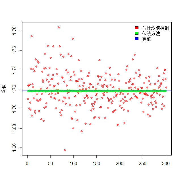
Average estimates：

Change in variance：

We can see that still as in the theoretical analysis, we can get a good estimation and an approximation to the tick function appears.

4. Conclusion

In the case where the true value \(\mu_y\) of the traditional control variable method is not known, we can use the additional data to estimate the mean value at \(Z_{cv}=X+c(Y-\mu_y)\) using the estimated amount \(\hat\mu_y\) instead. This gives us the relationship between the traditional control variable method of the method: \(MSE[Z_{cv}(c(k')),X]=MSE[\bar{\mu_x},X]\times[1-\rho^2(\frac{1}{1+\frac{k}{k'}})]\), which fits a generalized pairwise tick relationship. But we also find that only if the value of \(k'\) is large enough can we get a variance reduction that is almost consistent with the traditional control variable method, and when we can get the true value of \(\mu_y\), we still have to use the traditional control variable method.

Our use of this method makes it possible to extend the scope of our study even further, and to no longer just select control variables that know the true value, as long as we can The estimated variables are all optional.

5、 Further discussion

1. The introduction of control variables that are biased against the mean can be discussed further.
2. Does information about variance contribute to variance reduction in the control variable approach?

6、 references

[1]时蓬,杨明,刘飞.方差缩减中的控制变量方法研究[J].科学技术与工程,2011,11(22):5323-5327.

[2]Raghu Pasupathy,Bruce W. Schmeiser,Michael R. Taaffe,Jin Wang. Control-variate estimation using estimated control means[J]. IIE Transactions,2012,44(5).

[3]（美）SHELDON M.ROSS著；王兆军 陈广雷 邹长亮译.SIMULATION统计模拟 第4版[M].北京：人民邮电出版社.2007.