用TensorFlow实现一个在CIFAR-10数据集上80%准确率的卷积神经网络
本文主要介绍如何在TensorFlow上训练CIFAR-10数据集并达到80%的测试准确率。会涉及CIFAR-10数据处理、TensorFlow基本的卷积神经网络层(卷积层、池化层、激活函数等),所使用的代码没有经过仔细的封装,比较适合刚接触TensorFlow的同学,完整的代码可以在我的Github上下载:cifar10-CNN。
(PS:虽然网上有很多用TensorFlow训练CIFAR-10的博客或教程,但还是希望自己从头到尾写一遍,相当于学习笔记。)
预备知识
CIFAR-10数据集
CIFAR-10数据集的官网CIFAR,该数据集包含60000张32323的图片,包含10类常见物体。其中训练集50000张,测试集10000张。由于数据集规模比较适中,很适合初学者练习用。在训练模型的时候,常常会从训练集中抽出一小部分图片作为验证集以便于分析训练过程,防止出现过拟合的情况。官网还包含CIFAR-1OO数据集,有兴趣的可以直接看官网介绍,这里不多赘述。
关于数据下载,官网提供了3种版本:python版本、Matlab版本和二进制版本(适用于C语言),这里下载的是python版本。
TensorFlow中的常用层(卷积神经网络相关)
卷积层(2维)
卷积层用在卷积神经网络的前一部分,用于特征提取。
# import tensorflow as tf
tf.nn.conv2d(input, filter, strides, padding, use_cudnn_on_gpu=True, data_format='NHWC', name=None)
常用输入参数
- input: 4维张量(tensor),往往是输入图片或者上一层输出的特征图
- filter: 即滤波器,或者卷积核,卷积操作由卷积核在图像或者特征图上滑动计算完成
- strides: 卷积运算的步长,在二维卷积中,形如[1, s1, s2, 1]的格式
- padding: 指定图片边缘填充的方式,有"SAME"和"VALID"两种
池化层(2维)
池化最常见的是最大池化和平均池化,定义如下:
# import tensorflow as tf
tf.nn.max_pool(value, ksize, strides, padding, data_format='NHWC', name=None)
tf.nn.avg_pool(value, ksize, strides, padding, data_format='NHWC', name=None)
常用输入参数
- value: 4维张量(tensor),往往是卷积层输出的特征图
- ksize: 形如[1, s1, s2, 1]
- strides: 卷积运算的步长,在二维卷积中,形如[1, s1, s2, 1]的格式,即池化窗口大小
- stride: 步长,指定每次移动多少,与stride取不同的组合可以实现重叠池化和不重叠池化。
- padding: 指定图片边缘填充的方式,有"SAME"和"VALID"两种
全连接层
在典型的卷积神经网络中接在一系列卷积层后,用于根据卷积层提取的特征进行后续操作。全连接层在实现上是矩阵乘法。
#import tensorflow as tf
tf.matmul(a, b, transpose_a=False, transpose_b=False, adjoint_a=False, adjoint_b=False, a_is_sparse=False, b_is_sparse=False, name=None)
为了便于全连接的计算,往往会先把特征图平坦成一个一维的张量,这一步可以用TensorFlow中的reshape函数实现。
激活函数
激活函数赋予神经网络非线性变换的能力。Tensorflow中包含的激活函数很多,典型的激活函数如下:
# import tensorflow as tf
tf.nn.relu(features, name=None)
tf.nn.sigmoid(x, name=None)
tf.nn.tanh(x, name=None)
数据处理
前面提到过,训练的时候习惯从训练集中抽出一部分作为验证集。另外,模型的训练过程中,我们一般不会把所有的数据一次性全部读进来参与计算,而采用小批量的方式,即每次只抽取一部分的数据参与计算。所以这一部分主要介绍如何用python实现CIFAR-10数据集的下载、解析以及验证集的划分和小批量读取数据的实现。
数据下载
可以直接从官网上下载并解压,当然也可以利用python中的urllib模块和tarfile分别实现下载和解压。主要的函数如下:
def maybe_download_and_extract(url, download_dir):
    """
    Download and extract the data if it doesn't already exist.
    Assume the url is a tar-ball file

    Args:
        url: Internet URL for the tar-file to download.
        download_dir: Directory where the download file is saved.
    """

    filename = url.split('/')[-1]
    file_path = os.path.join(download_dir,filename)

    if not os.path.exists(file_path):
        if not os.path.exists(download_dir):
            os.mkdir(download_dir)
        """
        # for python2
        file_path, _ = urllib.urlretrieve(url=url,
                                          filename=file_path,
                                          reporthook=_print_download_progress)
        """
        # for python3
        file_path, _ = urllib.request.urlretrieve(url=url,
                                          filename=file_path,
                                          reporthook=_print_download_progress)
        print("download finished.")
    else:
        print("unpacking...")
        tarfile.open(name=file_path, mode='r:gz').extractall(download_dir)
        print("Data has apparently already been download and unpacked!")
考虑到python2和python3中urllib模块发生了一些改变,因此把两种实现都写在里面,可以根据自己的python版本选择。此外,里面还调用了一个用于显示下载进度的函数“reporthook=_print_download_progress”,具体定义如下:
def _print_download_progress(count, block_size, total_size):
    """
    function used for printing the download progress.
    Used as a call-back function in maybe_download_and_extract().
    """

    # percentage completion.
    pct_complete = float(count*block_size)/total_size

    # Status message.
    msg = "\r- Download progress: {0:.1%}".format(pct_complete) #'\r':当一行打印结束后,再从该行开始位置打印

    # Print
    sys.stdout.write(msg) # 相当于print(但最后不会添加换行符)
    sys.stdout.flush() # 输出缓冲,以便实时显示进度
经过上面下载和解压数据后,我们可以看到文件夹下一共包含以下文件:
- batches.meta: 解压后以列表存放了标签的名称,列表名是"label_names",即label_names[0] == “airplane”, label_names[1] == "automobile"等
- data+batch_1, … data+batch_5: 存放训练集(图片和标签),每个文件包含10000个数据
- test_batch: 测试集图片和标签,共10000个数据
- readme.html: 官网
解析数据
主要采用python的pickle模块解析数据,可以参考官网提供的函数:
python_version = sys.version[0]
data_path = os.getcwd()
data_path = os.path.join(data_path,'data/')
def _get_file_path(filename=''):
    """
    Return the full path of a data-file for the data-set.
    If filename=="" then return the directory of the files.
    """
    return os.path.join(data_path,'cifar-10-batches-py/', filename)

def _unpickle(filename):
    """
    Unpickle the given file and return the data.
    Note that the appropriate dir-name is prepended
    the filename.
    """
    file_path = _get_file_path(filename)
    print("Loading data: " + file_path)
    with open(file_path, mode='rb') as file:
        if python_version == "2":
            data = pickle.load(file)
        else:
            data = pickle.load(file, encoding="bytes")
    return data
需要注意的是,python2和3两个版本编码格式有所差异,所以上面的代码中加了Python版本判断。有了上面的一些辅助函数,我们就可以去解析数据文件:
def _convert_images(raw):
    """
    Convert images from unpickled data (10000, 3072)
    to a 4-dim array

    Args:
        raw: unpackled data from cifar10, eg: (10000,3072)
    return:
        a 4-dim array: (img_num, height, width, channel)
    """
    num_channels = 3
    img_size = 32
    raw_float = np.array(raw, dtype=float)/255.0
    images = raw_float.reshape([-1,num_channels,img_size,img_size])
    images = images.transpose([0, 2, 3, 1])
    return images

def _load_data(filename):
    """
    Load a pickled data-file from the CIFAR-10 data set
    and return the converted images (see above) and the
    class-number for each image.
    """
    data = _unpickle(filename)
    if python_version == "2":
        raw_images = data['data']
        labels = np.array(data['labels'])
    else:
        raw_images = data[b'data']
        labels = np.array(data[b'labels'])
    images = _convert_images(raw_images)
    return images, labels
filename可以是文件夹中的data_batch和test_batch。类似的方法我们可以解析出“batches.meta”中的标签名称:
def load_label_names():
    """
    Load the names for the classes in the CIFAR-10 data set.
    Returns a list with the names.
    Example: names[3] is the name associated with class-number 3.
    """
    raw = _unpickle("batches.meta")
    if python_version == "2":
        label_names = [x.decode('utf-8') for x in raw['label_names']]
    else:
        label_names = raw[b'label_names']
    return label_names
one-hot编码
在神经网络中,我们更倾向于对标签采用one-hot编码,因为这种方式在分类问题上更加方便合理。而上面函数返回的标签信息是0-9之间的数字(对用10个类别),因此需要对标签做one-hot编码:
def _one_hot_encoded(class_numbers, num_classes=None):
    """
    Generate the One-Hot encoded class-labels from an array of integers.

    For example, if class_number=2 and num_classes=4 then
    the one-hot encoded label is the float array: [0. 0. 1. 0.]

    Args:
        class_numbers: array of integers with class-numbers.
        num_classes: number of classes. If None then use max(cls)-1.
    Return:
        2-dim array of shape: [len(cls), num_classes]
    """
    if num_classes is None:
        num_classes = np.max(class_numbers)+1

    return np.eye(num_classes, dtype=float)[class_numbers]
对于上面的return语句,可能存在疑惑,这里举个例子便于理解:
import numpy as np
a = np.eye(10)
print("a = \n", a)
b = a[[1,3,5,7]]
print("b = \n", b)

'''输出结果:
a =
 [[1. 0. 0. 0. 0. 0. 0. 0. 0. 0.]
 [0. 1. 0. 0. 0. 0. 0. 0. 0. 0.]
 [0. 0. 1. 0. 0. 0. 0. 0. 0. 0.]
 [0. 0. 0. 1. 0. 0. 0. 0. 0. 0.]
 [0. 0. 0. 0. 1. 0. 0. 0. 0. 0.]
 [0. 0. 0. 0. 0. 1. 0. 0. 0. 0.]
 [0. 0. 0. 0. 0. 0. 1. 0. 0. 0.]
 [0. 0. 0. 0. 0. 0. 0. 1. 0. 0.]
 [0. 0. 0. 0. 0. 0. 0. 0. 1. 0.]
 [0. 0. 0. 0. 0. 0. 0. 0. 0. 1.]]
b =
 [[0. 1. 0. 0. 0. 0. 0. 0. 0. 0.]
 [0. 0. 0. 1. 0. 0. 0. 0. 0. 0.]
 [0. 0. 0. 0. 0. 1. 0. 0. 0. 0.]
 [0. 0. 0. 0. 0. 0. 0. 1. 0. 0.]]
'''
对比a和b的结果其实就很好理解了。首先,用numpy的eye()函数生成了一个10行10列的单位阵,然后我们给定一个索引列表[1,3,5,7],相当于把a的第1,3,5,7行抽出来赋值给了b。这样,b的每一行就分别对应1,3,5,7的one-hot标签,对应的位置为1。
载入训练集和测试集
有了上面的一些函数,我们就可以把CIFAR-1O所有的训练集和测试集都读进来了。对于训练集和测试集,不同之处在于训练集有5个文件,因此需要循环读取每一个文件最后再整个在一起。
def load_training_data():
    """
    Load all the training-data for the CIFAR-10 data-set.
    The data-set is split into 5 data-files which are merged here.

    Returns:
        images: training images
        labels: label of training images
        one_hot_labels: one-hot labels.
    """
    num_files_train = 5
    images_per_file = 10000
    num_classes = 10
    img_size = 32
    num_channels = 3
    num_images_train = num_files_train*images_per_file

    # 32bit的Python使用内存超过2G之后,此处会报MemoryError(最好用64位)
    images = np.zeros(shape=[num_images_train, img_size, img_size, num_channels], dtype=float)
    labels = np.zeros(shape=[num_images_train], dtype=int)

    begin = 0
    for i in range(num_files_train):
        images_batch, labels_batch = _load_data(filename="data_batch_"+str(i+1)) # _load_data2 in python2
        num_images = len(images_batch)
        end = begin + num_images
        images[begin:end,:] = images_batch
        labels[begin:end] = labels_batch
        begin = end
    one_hot_labels = _one_hot_encoded(class_numbers=labels,num_classes=num_classes)
    return images, labels, one_hot_labels

def load_test_data():
    """
    Load all the test-data for the CIFAR-10 data-set.
    Returns:
    the images, class-numbers and one-hot encoded class-labels.
    """
    num_classes = 10
    images, labels = _load_data(filename="test_batch") # _load_data2 in python2
    return images, labels, _one_hot_encoded(class_numbers=labels, num_classes=num_classes)
划分数据集
前面提高过,我们通常会从训练集中抽取一小部分数据作为验证集,以此来监督模型的训练过程或调整一些超参数。验证集的比例不用太大。这个过程最需要注意的是,在抽取图片的时候,要把对应的标签也抽取出来。一般的思路就是直接把训练集随机打乱,然后取出指定数量的数据,我的实现代码如下:
def split_train_data(images_train, one_hot_labels_train, ratio = 0.1, shuffle = False):
    """
    split valid data from train data with specified ratio.

    Arguments:
        images_train: train data (50000, 32, 32, 3).
        one_hot_labels_train: one-hot labels of train data (50000, 10).
        ratio: valid data ratio.
        shuffle: shuffle or not.
    Return:
        images_train: splitted train data.
        one_hot_labels_train: train data labels.
        images_valid: valid data
        one_hot_labels_valid: valid data labels
    """

    num_train = images_train.shape[0]
    num_valid = int(np.math.floor(num_train * ratio))

    if shuffle:
        permutation = list(np.random.permutation(num_train))
        images_train = images_train[permutation, ]
        one_hot_labels_train = one_hot_labels_train[permutation, ]

    images_valid = images_train[-num_valid:, ]
    one_hot_labels_valid = one_hot_labels_train[-num_valid:, ]
    images_train = images_train[0:-num_valid, ]
    one_hot_labels_train = one_hot_labels_train[0:-num_valid, ]
    return images_train, one_hot_labels_train, images_valid, one_hot_labels_valid
上面的代码中用到了numpy库中的random模块。举个例子,假设我想生成一个1至10的随机序列,可以这么干:
from numpy.random import permutation
p = list(permutation(10))
print(p)
# [5, 8, 7, 0, 9, 6, 4, 1, 2, 3] (也可能是其他排序)
利用上面的原理,我们就可以随机打乱训练图片和标签。补充一点,随机打乱数据不仅仅可以用在划分训练集和验证集上,还可以用于训练过程中。典型的做法是当模型遍历完一边训练样本后(1个epoch),重新打乱训练样本,这样做的好处是保证每个epoch抽到的mini batch都是随机的,可以提高模型的泛化能力。
生成mini-batch
有两种思路:第一种是每次训练的时候都从训练集中随机抽取一个mini-batch的数据,这种思路实现起来很简单,但存在一个问题,在训练过程中不能保证所有的训练样本都被抽到。即很有可能有的样本被抽到很多次,而有的样本可能一次也抽不到。第二中思路是先对整个训练集进行随机打乱,然后依次取出一个mini-batch的数据,等到所有的数据都被训练了一次(1个epoch),重新打乱数据,执行相同操作。这样做虽然保证了均匀采样,但需要提前把所有数据一次性读入内存,比较占用资源。这里我以第二种思路编写函数如下:
def create_mini_batches(X, Y, mini_batch_size = 128, shuffle=False):
    """
    Create a list of minibatches from the training images.

    Arguments:
        X: numpy.ndarry images shaped (num_images, height, width, channels).
           for example: (50000, 32, 32, 3).
        Y: one-hot labels of images shaped (num_images, num_classes).
           for example: (50000,10)
        mini_batch_size: Mini-batch size .
        shuffle: Shuffling the images or not.
    Return:
        mini_batches_X: a list of all mini-batches images, each element in
                        it is an numpy.ndarray containing one batch of images.
        mini_batches_Y: a list of all mini-batches one-hot labels,
                        each element in it is an one-hot label.
    """
    m = X.shape[0]
    mini_batches_X = []
    mini_batches_Y = []

    if shuffle:
        permutation = list(np.random.permutation(m))
        X = X[permutation, ]
        Y = Y[permutation, ]

    num_complete_minibathes = int(np.math.floor(m/mini_batch_size))

    for k in range(0, num_complete_minibathes):
        mini_batch_X = X[k*mini_batch_size:(k+1)*mini_batch_size, ]
        mini_batch_Y = Y[k*mini_batch_size:(k+1)*mini_batch_size, ]

        mini_batches_X.append(mini_batch_X)
        mini_batches_Y.append(mini_batch_Y)

    if m % mini_batch_size != 0:
        mini_batch_X = X[num_complete_minibathes*mini_batch_size:, ]
        mini_batch_Y = Y[num_complete_minibathes*mini_batch_size:, ]
        mini_batches_X.append(mini_batch_X)
        mini_batches_Y.append(mini_batch_Y)

    return mini_batches_X, mini_batches_Y
模型
这里一共介绍两个模型,一个是AlexNet风格的模型cifar10_5layers,共5层,另一个是VGG风格的模型cifar10_8layers,共8层。考虑到时间成本和硬件条件,模型中的输出输出维度取值比较小。为了代码的简洁,先封装几个函数,如下:
def max_pool(feature_map):
    return tf.nn.max_pool(feature_map, ksize=[1, 2, 2, 1], strides=[1, 2, 2, 1], padding='SAME')

def conv_relu(feature_map, weight, bias):
    conv = tf.nn.conv2d(feature_map, weight, strides=[1, 1, 1, 1], padding='SAME')
    return tf.nn.relu(conv + bias)

def conv_pool_relu(feature_map, weight, bias):
    conv = tf.nn.conv2d(feature_map, weight, strides=[1, 1, 1, 1], padding='SAME')
    pool = tf.nn.max_pool(conv, ksize=[1, 2, 2, 1], strides=[1, 2, 2, 1], padding='SAME')
    return tf.nn.relu(pool + bias)

def fc_relu(fc_input, weight, bias):
    fc = tf.matmul(fc_input, weight)
    return tf.nn.relu(fc + bias)
模型中卷积步长都取1,padding为“SAME”;采用最大池化,窗口大小为2×2,步长为2;因此每次卷积不改变特征图大小,每次池化使特征图尺寸缩减一半。
cifar10_5layers
因为在实验中打算尝试不同的初始化方法,因此在模型定义的时候把模型初始化方法定义成一个参数。其他地方应该很直观,就不介绍了。
def cifar10_5layers(input_image, keep_prob, init_method=tf.truncated_normal_initializer(stddev=1e-2)):
    """
    model definition with 5 layers.

    Args:
        input_image: input image tensor.
        init_method: initialization method.
                     The default is tf.truncated_normal_initializer(1e-2)
    Return:
        model: computation graph of the defined model.
    """
    with tf.variable_scope("conv1"):
        W1 = tf.get_variable(name="W1", shape=[5,5,3,32], dtype=tf.float32, \
                             initializer=init_method)
        b1 = tf.get_variable(name="b1", shape=[32], dtype=tf.float32, \
                             initializer=tf.constant_initializer(0.01))
        conv1 = conv_pool_relu(input_image, W1, b1)
    with tf.variable_scope("conv2"):
        W2 = tf.get_variable(name="W2", shape=[5,5,32,64], dtype=tf.float32, \
                             initializer=init_method)
        b2 = tf.get_variable(name="b2", shape=[64], dtype=tf.float32, \
                             initializer=tf.constant_initializer(0.01))
        conv2 = conv_pool_relu(conv1, W2, b2)
	conv2 = tf.nn.dropout(conv2, keep_prob)
    with tf.variable_scope("conv3"):
        W3 = tf.get_variable(name="W3", shape=[5,5,64,128], dtype=tf.float32, \
                             initializer=init_method)
        b3 = tf.get_variable(name="b3", shape=[128], dtype=tf.float32, \
                             initializer=tf.constant_initializer(0.01))
        conv3 = conv_pool_relu(conv2, W3, b3)
	conv3 = tf.nn.dropout(conv3, keep_prob)
    with tf.variable_scope("fc1"):
        W4 = tf.get_variable(name="W4", shape=[4*4*128,256], dtype=tf.float32, \
                             initializer=init_method)
        b4 = tf.get_variable(name="b4", shape=[256], dtype=tf.float32, \
                             initializer=tf.constant_initializer(0.01))
        conv3_flat = tf.reshape(conv3, [-1, 4*4*128])
        fc1 = fc_relu(conv3_flat, W4, b4)
	fc1 = tf.nn.dropout(fc1, keep_prob)
    with tf.variable_scope("output"):
        W5 = tf.get_variable(name="W5", shape=[256,10], dtype=tf.float32, \
                             initializer=init_method)
        b5 = tf.get_variable(name="b5", shape=[10], dtype=tf.float32, \
                             initializer=tf.constant_initializer(0.01))
	y_logit = tf.matmul(fc1, W5) + b5
    return y_logit, tf.nn.softmax(y_logit, name="softmax")
cifar10_8layers
def cifar10_8layers(input_image, keep_prob, init_method=tf.truncated_normal_initializer()):
    """
    model definition with 8 layers.

    Args:
        input_image: input image tensor.
        init_method: initialization method.
                     The default is tf.truncated_normal_initializer()
        keep_prop: keep propobality in dropout.
    Return:
        model: computation graph of the defined model.
    """
    with tf.variable_scope("conv1_1"):
        W1_1 = tf.get_variable(name="W1_1", shape=[3,3,3,32], dtype=tf.float32, \
                             initializer=init_method)
        b1_1 = tf.get_variable(name="b1_1", shape=[32], dtype=tf.float32, \
                             initializer=tf.constant_initializer(0.01))
        conv1_1 = conv_relu(input_image, W1_1, b1_1)
    with tf.variable_scope("conv1_2"):
        W1_2 = tf.get_variable(name="W1_2", shape=[3,3,32,32], dtype=tf.float32, \
                             initializer=init_method)
        b1_2 = tf.get_variable(name="b1_2", shape=[32], dtype=tf.float32, \
                             initializer=tf.constant_initializer(0.01))
        conv1_2 = max_pool(conv_relu(conv1_1, W1_2, b1_2))
    with tf.variable_scope("conv2_1"):
        W2_1 = tf.get_variable(name="W2_1", shape=[3,3,32,64], dtype=tf.float32, \
                             initializer=init_method)
        b2_1 = tf.get_variable(name="b2_1", shape=[64], dtype=tf.float32, \
                             initializer=tf.constant_initializer(0.01))
        conv2_1 = conv_relu(conv1_2, W2_1, b2_1)
    with tf.variable_scope("conv2_2"):
        W2_2 = tf.get_variable(name="W2_2", shape=[3,3,64,64], dtype=tf.float32, \
                             initializer=init_method)
        b2_2 = tf.get_variable(name="b2_2", shape=[64], dtype=tf.float32, \
                             initializer=tf.constant_initializer(0.01))
        conv2_2 = max_pool(conv_relu(conv2_1, W2_2, b2_2))
    with tf.variable_scope("conv3_1"):
        W3_1 = tf.get_variable(name="W3_1", shape=[3,3,64,128], dtype=tf.float32, \
                             initializer=init_method)
        b3_1 = tf.get_variable(name="b3_1", shape=[128], dtype=tf.float32, \
                             initializer=tf.constant_initializer(0.01))
        conv3_1 = conv_relu(conv2_2, W3_1, b3_1)
    with tf.variable_scope("conv3_2"):
        W3_2 = tf.get_variable(name="W3_2", shape=[3,3,128,128], dtype=tf.float32, \
                             initializer=init_method)
        b3_2 = tf.get_variable(name="b3_2", shape=[128], dtype=tf.float32, \
                             initializer=tf.constant_initializer(0.01))
        conv3_2 = max_pool(conv_relu(conv3_1, W3_2, b3_2))
        conv3_2 = tf.nn.dropout(conv3_2, keep_prob)
    with tf.variable_scope("fc1"):
        W4 = tf.get_variable(name="W4", shape=[4*4*128,256], dtype=tf.float32, \
                             initializer=init_method)
        b4 = tf.get_variable(name="b4", shape=[256], dtype=tf.float32, \
                             initializer=tf.constant_initializer(0.01))
        conv3_flat = tf.reshape(conv3_2, [-1, 4*4*128])
        fc1 = fc_relu(conv3_flat, W4, b4)
        fc1 = tf.nn.dropout(fc1, keep_prob)
    with tf.variable_scope("fc2"):
        W5 = tf.get_variable(name="W5", shape=[256,512], dtype=tf.float32, \
                             initializer=init_method)
        b5 = tf.get_variable(name="b5", shape=[512], dtype=tf.float32, \
                             initializer=tf.constant_initializer(0.01))
        fc2 = fc_relu(fc1, W5, b5)
        fc2 = tf.nn.dropout(fc2, keep_prob)
    with tf.variable_scope("output"):
        W6 = tf.get_variable(name="W6", shape=[512,10], dtype=tf.float32, \
                             initializer=init_method)
        b6 = tf.get_variable(name="b6", shape=[10], dtype=tf.float32, \
                             initializer=tf.constant_initializer(0.01))
        y_logit = tf.matmul(fc2, W6) + b6
    return y_logit, tf.nn.softmax(y_logit, name="softmax")
训练
训练模型的相关代码在train.py文件中。实验一共考虑了三种初始化方法即正太分布、Xavier初始化和He初始化,如下:
init_methods = {"Gaussian": tf.truncated_normal_initializer(stddev=1e-2),
                "Xavier": tf.contrib.layers.xavier_initializer_conv2d(),
                "He": tf.contrib.layers.variance_scaling_initializer()}
为了方便调用不同的模型和初始化方法,代码中通过解析命令行输入来获取相应的参数:
def parse_args():
	"""
	parse input arguments.
	"""
	parse = argparse.ArgumentParser(description="CIFAR-10 training")
	parse.add_argument("--model", dest="model_name",
					   help="model name: 'cifar10-5layers' or 'cifar10-8layers'",
					   default="cifar10-5layers")
	parse.add_argument("--init", dest="init_method",
					   help="initialization method for weights, 'Gaussian', 'Xavier' or 'He'",
					   default="Gaussian")
	args = parse.parse_args() # 获取所有的参数
	return args
在构建模型的时候,就可以根据命令行参数来定义我们需要的模型:
args = parse_args()
# ...
# 创建模型
X = tf.placeholder(tf.float32, [None, img_size, img_size, num_channels])
Y_ = tf.placeholder(tf.float32, [None, num_classes])
keep_prob = tf.placeholder(tf.float32)

init_method = init_methods[args.init_method]
if args.model_name == "cifar10-5layers":
    logit, Y = cifar10_5layers(X, keep_prob, init_method)
elif args.model_name == "cifar10-8layers":
    logit, Y = cifar10_8layers(X, keep_prob, init_method)
模型定义好后,还需要指定损失函数和学习方法才能训练:
# 交叉熵损失和准确率
cross_entropy = tf.nn.softmax_cross_entropy_with_logits(logits=logit, labels=Y_)
cross_entropy = tf.reduce_mean(cross_entropy)
correct_prediction = tf.equal(tf.argmax(Y, 1), tf.argmax(Y_, 1))
accuracy = tf.reduce_mean(tf.cast(correct_prediction, tf.float32))
# ...
lr = 0.0001
train_step = tf.train.AdamOptimizer(lr).minimize(cross_entropy)
init = tf.global_variables_initializer()
训练过程中,为了提高模型的鲁棒性,在每次遍历一遍训练集后就重新打乱一次训练数据,如下:
with tf.Session() as sess:
    # ...
    for i in range(train_steps+1):
        # 获取一个mini batch数据
        j = i%num_batches # j用于记录第几个mini batch
        batch_X = images_train_batches[j]
        batch_Y = labels_train_batches[j]
        if j == num_batches-1: # 遍历一遍训练集(1个epoch)
            images_train_batches, labels_train_batches = create_mini_batches(images_train, \
                                                                            labels_train, \
                                                                            shuffle=True)
        # ...
注意,在训练阶段,需要指定drop参数keep_prob=0.5,而在测试阶段指定为1:
sess.run(fetches=train_step, feed_dict={X: batch_X, Y_: batch_Y, keep_prob: 0.5})
模型训练过程中,每训练一定的次数,我们保存一次中间结果:
saver = tf.train.Saver()
# ...
with tf.Session() as sess:
    for i in range(train_steps+1):
        if i % 10000 == 0 and i > 0:
            model_name = args.model_name + "_" + args.init_method
            model_name = os.path.join("./models", model_name)
            saver.save(sess, model_name, global_step=i)
还有其他的一些细节,比如保存训练日志等,这里就不一一介绍,可以看具体的代码实现。
测试
我们需要在测试集上来检验训练好的模型的性能,大致过程为重新构建模型、读取训练好的权重,输入测试数据计算准确率,代码如下:
#coding: utf-8
from __future__ import print_function
import tensorflow as tf
from model import cifar10_5layers, cifar10_8layers
from cifar10 import load_test_data
import os
import argparse

def parse_args():
    	"""
	parse input arguments.
	"""
	parse = argparse.ArgumentParser(description="CIFAR-10 test")
	parse.add_argument("--model", dest="model_name",
					   help="model name: 'cifar10-5layers' or 'cifar10-8layers'",
					   default="cifar10-5layers")
	parse.add_argument("--path", dest="model_path",
					   help="trained model file path: ***.data***",
					   default="models/cifar10-5layers_Gaussian-10000.data-00000-of-00001")
	args = parse.parse_args()
	return args


def main():
    args = parse_args()
    model_name = args.model_name
    model_path = args.model_path.split(".")[0]
    # 加载测试数据集
    images_test, _, labels_test = load_test_data()
    print("images_test.shape = ", images_test.shape)

    # 构建模型(模型也可以直接从.meta文件中恢复)
    X = tf.placeholder(tf.float32, [None, 32, 32, 3])
    Y_ = tf.placeholder(tf.float32, [None, 10])
    keep_prob = tf.placeholder(tf.float32)
    if model_name == "cifar10-5layers":
        _, Y = cifar10_5layers(X, keep_prob)
    elif model_name == "cifar10-8layers":
        _, Y = cifar10_8layers(X, keep_prob)
    else:
        print("wrong model name!")
        print("model name: 'cifar10-5layers' or 'cifar10-8layers'")
        raise KeyError

    correct_prediction = tf.equal(tf.argmax(Y, 1), tf.argmax(Y_, 1))
    accuracy = tf.reduce_mean(tf.cast(correct_prediction, tf.float32))

    saver = tf.train.Saver()
    with tf.Session() as sess:
        # 恢复模型权重
        saver.restore(sess, model_path)
        # 测试,注意测试阶段keep_prob=1
        print("test accuracy = ", sess.run(accuracy, feed_dict={X: images_test, Y_: labels_test, keep_prob: 1}))

if __name__ == "__main__":
    main()
其实我们在训练阶段不仅保存了模型的权重,还保存了模型整个结构图,因此,不一定要重新定义一个相同的模型,只需要从保存的结构图中恢复即可,有关这块内容更详细的介绍可以参考这篇博客:
一份快速完整的Tensorflow模型保存和恢复教程(译)
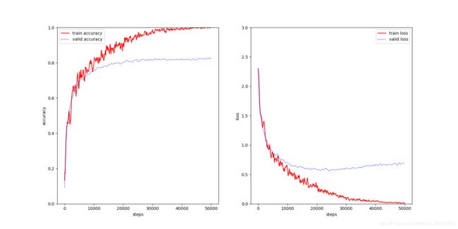
实验结果
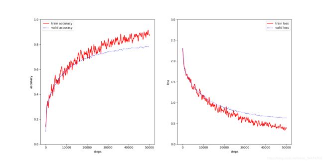
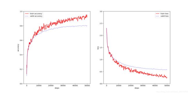
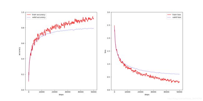
cifar10_5layers
-
正太分布(高斯初始化)
-
Xavier初始化
-
He初始化
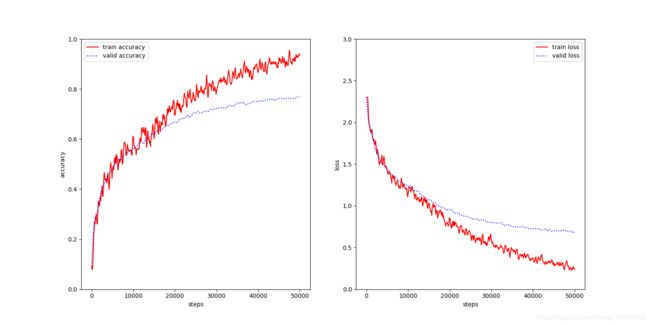
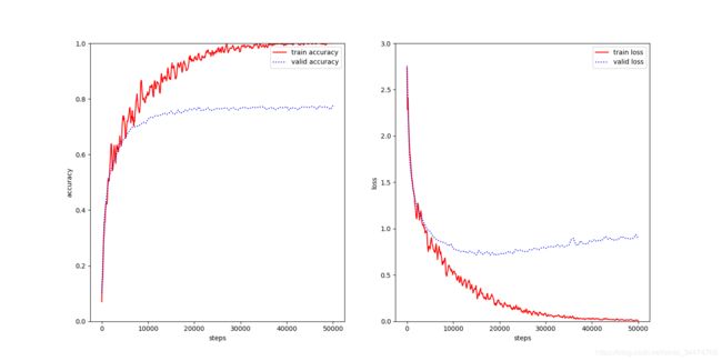
cifar10_8layers
-
正太分布(高斯初始化)
-
Xavier初始化
-
He初始化
测试集上准确率
| 模型 | 5层正态 | 5层Xavier | 5层He | 8层正态 | 8层Xavier | 8层He |
|---|---|---|---|---|---|---|
| 准确率 | 78.14% | 80.81% | 79.68% | 75.52% | 81.75% | 77.03% |
总结
本篇博客主要总结了本人在CIFAR-10数据集上的训练和测试过程,所训练的模型在测试集上达到80%的准确率。由于能力和精力有限,不能做到尽善尽美,仍有许多不足之处:
- 数据读取速度较慢,占有内存较大。 在数据处理和读取部分,数据集是一次性读到内存中,在训练阶段进行每一个批次的读取。如果能利用多线程机制(如TensorFlow中提供的队列和多线程机制),可以显著提高数据的读取速度并降低内存消耗。
- 模型普遍过拟合。 其实在采用5层的网络训练的时候已经出现了过拟合现象,在8层网络的时候更严重。这一点是由于模型设计不合理和数据集较小导致的(训练集中还划分出一部分验证集)。比较简单的一个缓解措施是对训练集进行扩充,平移、翻转、裁剪、亮度变换等。有兴趣的同学可以自己尝试(可以使用TensorFlow快速实现图像扩充)
写在最后的话:
感谢你一直读到这里,希望本篇博客对你有点帮助。关于本篇博客中的任何问题欢迎指出,虚心接受各位大佬的教导!