__Sunshine__

论文阅读笔记（四十四）：Deconvolutional Networks

Building robust low and mid-level image representations, beyond edge primitives, is a long-standing goal in vision. Many existing feature detectors spatially pool edge information which destroys cues such as edge intersections, parallelism and symmetry. We present a learning framework where features that capture these mid-level cues spontaneously emerge from image data. Our approach is based on the convolutional decomposition of images under a sparsity constraint and is totally unsupervised. By building a hierarchy of such decompositions we can learn rich feature sets that are a robust image representation for both the analysis and synthesis of images.

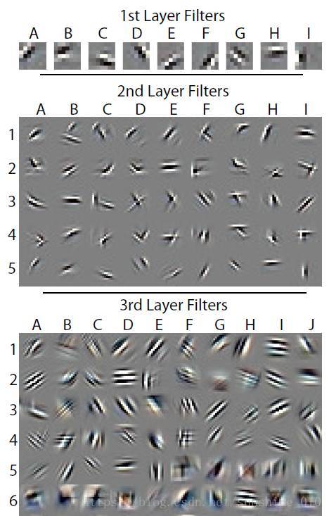
In this paper we propose Deconvolutional Networks, a framework that permits the unsupervised construction of hierarchical image representations. These representations can be used for both low-level tasks such as denoising, as well as providing features for object recognition. Each level of the hierarchy groups information from the level beneath to form more complex features that exist over a larger scale in the image. Our grouping mechanism is sparsity: by encouraging parsimonious representations at each level of the hierarchy, features naturally assemble into more complex structures. However, as we demonstrate, sparsity itself is not enough – it must be deployed within the correct architecture to have the desired effect. We adopt a convolutional approach since it provides stable latent representations at each level which preserve locality and thus facilitate the grouping behavior. Using the same parameters for learning each layer, our Deconvolutional Network (DN) can automatically extract rich features that correspond to mid-level concepts such as edge junctions, parallel lines, curves and basic geometric elements, such as rectangles. Remarkably, some of them look very similar to the mid-level tokens posited by Marr in his primal sketch theory [18] (see Fig. 1).

Our proposed model is similar in spirit to the Convolutional Networks of LeCun et al. [13], but quite different in operation. Convolutional networks are a bottom-up approach where the input signal is subjected to multiple layers of convolutions, non-linearities and sub-sampling. By contrast, each layer in our Deconvolutional Network is top-down; it seeks to generate the input signal by a sum over convolutions of the feature maps (as opposed to the input) with learned filters. Given an input and a set of filters, inferring the feature map activations requires solving a multi-component deconvolution problem that is computationally challenging. In response, we use a range of tools from low-level vision, such as sparse image priors and efficient algorithms for image deblurring. Correspondingly, our paper is an attempt to link high-level object recognition with low-level tasks like image deblurring through a unified architecture.

Related Work
Deconvolutional Networks are closely related to a number of “deep learning” methods [2, 8] from the machine learning community that attempt to extract feature hierarchies from data. Deep Belief Networks (DBNs) [8] and hierarchies of sparse auto-encoders [22, 9, 26], like our approach, greedily construct layers from the image upwards in an unsupervised fashion. In these approaches, each layer consists of an encoder and decoder. The encoder provides a bottom-up mapping from the input to latent feature space while the decoder maps the latent features back to the input space, hopefully giving a reconstruction close to the original input. Going from the input directly to the latent representation without using the encoder is difficult because it requires solving an inference problem (multiple elements in the latent features are competing to explain each part of the input). As these models have been motivated to improve high-level tasks like recognition, an encoder is needed to perform fast, but highly approximate, inference to compute the latent representation at test time. However, during training the latent representation produced by performing top-down inference with the decoder is constrained to be close to the output of the encoder. Since the encoders are typically simple non-linear functions, they have the potential to significantly restrict the latent representation obtainable, producing sub-optimal features. Restricted Boltzmann Machines (RBM), the basic module of DBNs, have the additional constraint that the encoder and decoder must share weights. In Deconvolutional Networks, there is no encoder: we directly solve the inference problem by means of efficient optimization techniques. The hope is that by computing the features exactly (instead of approximately with an encoder) we can learn superior features.

Figure 1. (a): “Tokens” from Fig. 2-4 of Vision by D. Marr [18]. These idealized local groupings are proposed as an intermediate level of representation in Marr’s primal sketch theory. (b): Selected filters from the 3rd layer of our Deconvolutional Network, trained in an unsupervised fashion on real-world images.

Most deep learning architectures are not convolutional, but recent work by Lee et al. [15] demonstrated a convolutional RBM architecture that learns high-level image features for recognition. This is the most similar approach to our Deconvolutional Network, with the main difference being that we use a decoder-only model as opposed to the symmetric encoder-decoder of the RBM.

Our work also has links to recent work in sparse image decompositions, as well as hierarchical representations. Lee et al. [14] and Mairal et al. [16, 17] have proposed efficient schemes for learning sparse over-complete decompositions of image patches [19], using a convex L1 sparsity term. Our approach differs in that we perform sparse decomposition over the whole image at once, not just for small image patches. As demonstrated by our experiments, this is vital if rich features are to be learned. The key to making this work efficiently is to use a convolutional approach.

A range of hierarchical image models have been proposed. Particularly relevant is the work of Zhu and colleagues [31, 25], in particular Guo et al. [7]. Here, edges are composed using a hand-crafted set of image tokens into large-scale image structures. Grouping is performed via basis pursuit with intricate splitting and merging operations on image edges. The stochastic image grammars of Zhu and Mumford [31] also use fixed image primitives, as well as a complex Markov Chain Monte-Carlo (MCMC)-based scheme to parse scenes. Our work differs in two important ways: first, we learn our image tokens completely automatically. Second, our inference scheme is far simpler than either of the above frameworks.

Zhu et al. [30] propose a top-down parts-and-structure model but it only reasons about image edges, as provided by a standard edge detector, unlike ours which directly operates on pixels. The biologically inspired HMax model of Serre et al. [24, 23] use exemplar templates in their intermediate representations, rather than learning conjunctions of edges as we do. Fidler and Leonardis [5, 4] propose a top-down model for object recognition which has an explicit notion of parts whose correspondence is explicitly reasoned about at each level. In contrast, our approach simply performs a low-level deconvolution operation at each level, rather than attempting to solve a correspondence problem. Amit and Geman [1] and Jin and Geman [10] apply hierarchical models to deformed Latex digits and car license plate recognition.

Model
We first consider a single Deconvolutional Network layer applied to an image. This layer takes as input an image yi, composed of K0 color channels y1i , … , yi . We represent K0 each channel c of this image as a linear sum of K1 latent feature maps zik convolved with filters fk,c:

Henceforth, unless otherwise stated, symbols correspond to matrices. If yci is an Nr ×Nc image and the filters are H ×H , then the latent feature maps are (Nr +H −1)×(Nc +H −1) in size. But Eqn. 1 is an under-determined system, so to yield a unique solution we introduce a regularization term on zik that encourages sparsity in the latent feature maps. This gives us an overall cost function of the form:

where we assume Gaussian noise on the reconstruction term and some sparse norm p for the regularization. Note that the sparse norm |w|p is actually the p-norm on the vectorized version of matrix w, i.e. |w|p = i,j |w(i, j)|p. Typically, p = 1, although other values are possible, as described in Section 3.2. λ is a constant that balances the relative contributions of the reconstruction of yi and the sparsity of the feature maps zik .

Note that our model is top-down in nature: given the latent feature maps, we can synthesize an image. But unlike the sparse auto-encoder approach of Ranzato et al. [21], or DBNs [8], there is no mechanism for generating the feature maps from the input, apart from minimizing the cost function C1 in Eqn. 2. Many approaches focus on bottom-up inference, but we concentrate on obtaining high quality latent representations.

In learning, described in Section 3.2, we use a set of images y = {y1,…,yI} for which we seek argminf,zC1(y)2 , the latent feature maps for each image and the filters. Note that each image has its own set of feature maps while the filters are common to all images.

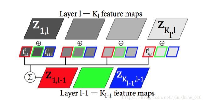
Figure 2. A single Deconvolutional Network layer (best viewed in color). For clarity, only the connectivity for a single input map is shown. In practice the first layer is fully connected, while the connectivity of the higher layers is specified by the map gl, which is sparse.

Forming a hierarchy
The architecture described above produces sparse feature maps from a multi-channel input image. It can easily be stacked to form a hierarchy by treating the feature maps zik,l of layer l as input for layer l + 1. In other words, layer l has as its input an image with Kl−1 channels being the number of feature maps at layer l − 1. The cost function Cl for layer l is a generalization of Eqn. 2, being:

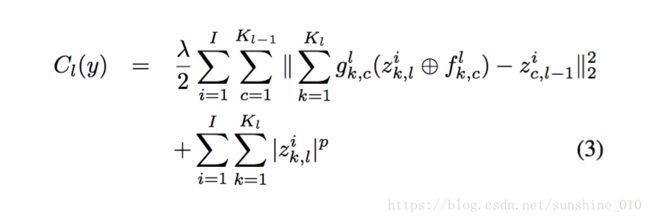
where zic,l−1 are the feature maps from the previous layer, and glk,c are elements of a fixed binary matrix that determines the connectivity between the feature maps at successive layers, i.e. whether zik,l is connected to zik,l−1 or not k,l c,l−1[13]. In layer-1 we assume that g1k,c is always 1, but in higher layers it will be sparse. We train the hierarchy from the bottom upwards, thus zik,l−1 is given from the results of learning on Cl−1(y). This structure is illustrated in Fig. 2.

Unlike several other hierarchical models [15, 21, 9] we do not perform any pooling, sub-sampling or divisive normalization operations between layers, although they could easily be incorporated.

Learning filters
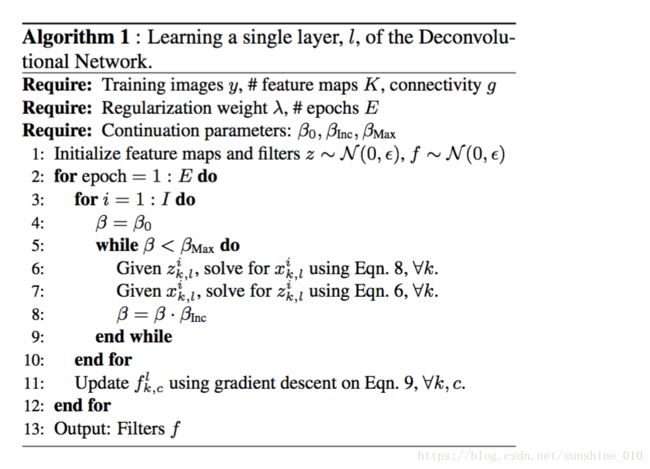
To learn the filters, we alternately minimize Cl(y) over the feature maps while keeping the filters fixed (i.e. perform inference) and then minimize Cl(y) over the filters while keeping the feature maps fixed. This minimization is done in a layer-wise manner starting with the first layer where the inputs are the training images y. Details are given in Algorithm 1. We now describe how we learn the feature maps and filters by introducing a framework suited for large scale problems.

Inferring feature maps: Inferring the optimal feature maps zik,l , given the filters and inputs is the crux of our approach. The sparsity constraint on zik,l which prevents the k,l model from learning trivial solutions such as the identity function. When p = 1 the minimization problem for the feature maps is convex and a wide range of techniques have been proposed [3, 14]. Although in theory the global minimum can always be found, in practice this is difficult as the problem is very poorly conditioned. This is due to the fact that elements in the feature maps are coupled to one another through the filters. One element in the map can be affected by another distant element, meaning that the minimization can take a very long time to converge to a good solution.

We tried a range of different minimization approaches to solve Eqn. 3, including direct gradient descent, Iterative Reweighted Least Squares (IRLS) and stochastic gradient descent. We found that direct gradient descent suffers from the usual problem of flat-lining and thereby gives a poor solution. IRLS is too slow for large-scale problems with many input images. Stochastic gradient descent was found to require many thousands of iterations for convergence.

Instead, we introduce a more general framework that is suitable for any value of p > 0, including pseudo-norms where p < 1. The approach is a type of continuation method, as used by Geman [6] and Wang et al. [27]. Instead of optimizing Eqn. 3 directly, we minimize an auxiliary cost function Cˆl(y) which incorporates auxiliary variables xi k,l for each element in the feature maps zik,l :

where β is a continuation parameter. Introducing the auxiliary variables separates the convolution part of the cost function from the | · |p term. By doing so, an alternating form of minimization for zik,l can be used. We first fix xik,l yielding a quadratic problem in zik,l . Then, we fix zik,l and solve a separable 1D problem for each element in xik,l . We call these two stages the z and x sub-problems respectively.

Filter updates : With x fixed and zik,l computed for a fixed i, we use the following for gradient updates of flk,c :

where Z is a convolution matrix similar to F . The overall
learning procedure is summarized in Algorithm 1.

Image representation/reconstruction
To use the model for image reconstruction, we first decompose an input image by using the learned filters f to find the latent representation z. We explain the procedure for a 2 layer model. We first infer the feature maps zk,1 for layer 1 using the input y′ and the filters f1k,c by minimizing ′ k,c C1(y ). Next we update the feature maps for layer 2, zk,2 in an alternating fashion. In step 1, we first minimize the reconstruction error w.r.t. y′, projecting zk,2 through f2k,c and f1k,c to the image:

In step 2, we minimize the error w.r.t. zk,2 :

We alternate between steps 1 and 2, using conjugate gradient descent in both. Once zk,2 has converged, we reconstruct y′ by projecting back to the image via f2k,c and f1k,c :

An important detail is the addition of an extra feature map z0 per input map of layer 1 that connects to the image via a constant uniform filter f0. Unlike the sparsity priors on the other feature maps, z0 has an l2 prior on the gradients of z0 , i.e. the prior is of the form ∥∇z0 ∥2 . These maps capture the low-frequency components, leaving the high-frequency edge structure to be modeled by the learned filters. Given that the filters were learned on high-pass filtered images, the z0 maps assist in reconstructing raw images.

Denoising images

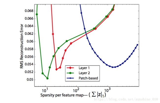
Figure 6. Exploring the trade-off between sparsity and denoising performance for our 1st and 2nd layer representations (red and green respectively), as well as the patch-based approach of Mairal et al. [16] (blue). Our 2nd layer representation simultaneously achieves a lower reconstruction error and sparser feature maps.

Given that our learned representation can be used for synthesis as well as analysis, we explore the ability of a two layer model to denoise images. Applying Gaussian noise to an image with a SNR of 13.84dB, the first layer of our model was able to reduce the noise to 16.31dB. Further, using the latent features of our second layer to reconstruct the image, the noise was reduced to a SNR of 18.01dB.

We also explore the relative sparsity of the feature maps in the 1st and 2nd layers of our model as we vary λ. In Fig. 6 we plot the average sparsity of each feature map against RMS reconstruction error, we see that the feature maps at layer 2 are sparser and give a lower reconstruction error, than those of layer 1. We also plot the same curve for the patch-based sparse decomposition of Mairal et al. [16]. In this framework, inference is performed separately for each image patch and since patches overlap, a much larger number of latent features are needed to represent the image. The curve was produced by varying the number of active dictionary atoms per patch in reconstruction.

Conclusion
We have introduced Deconvolutional Networks: a conceptually simple framework for learning sparse, overcomplete feature hierarchies. Applying this framework to natural images produces a highly diverse set of filters that capture high-order image structure beyond edge primitives. These arise without the need for hyper-parameter tuning or additional modules, such as local contrast normalization, max-pooling and rectification [9]. Our approach relies on robust optimization techniques to minimize the poorly conditioned cost functions that arise in the convolutional setting. Supplemental images, video, and code can be found at: http://www.cs.nyu.edu/ ̃zeiler/ pubs/cvpr2010/.

论文阅读笔记（四十四）：Deconvolutional Networks

你可能感兴趣的:(笔记)