02_End-to-End Machine Learning Project_StratifiedShuffleSplit_RMSE_MAE_Geographical Data_CaliforniaH
Here are the main steps you will go through:
1. Look at the big picture.
2. Get the data.
3. Discover and visualize the data to gain insights.
4. Prepare the data for Machine Learning algorithms.
5. Select a model and train it.
6. Fine-tune your model.
7. Present your solution.
8. Launch, monitor, and maintain your system
1.Look at the Big Picture
The first task you are asked to perform is to build a model of housing prices in California using the California census人口普查 data. This data has metrics such as the population, median income, median housing price, and so on for each block group in California. Block groups are the smallest geographical unit for which the US Census Bureau publishes sample data (a block
group typically has a population of 600 to 3,000 people). We will just call them “districts” for short.
Your model should learn from this data and be able to predict the median housing price in any district, given all the other metrics.
Frame the Problem
The first question to ask your boss is what exactly is the business objective; building a model is probably not the end goal. How does the company expect to use and benefit from this model? This is important because it will determine how you frame the problem, what algorithms you will select, what performance measure you will use to evaluate your model, and how much effort you should spend tweaking it.
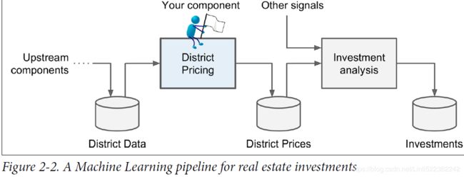
Your boss answers that your model’s output (a prediction of a district’s median housing price) will be fed to another Machine Learning system (see Figure 2-2), along with many other signals. This downstream system will determine whether it is worth investing in a given area or not. Getting this right is critical, as it directly affects revenue.
##################################################################################################
Pipelines
A sequence of data processing components is called a data pipeline. Pipelines are very common in Machine Learning systems, since there is a lot of data to manipulate and many data transformations to apply.
Components typically run asynchronously. Each component pulls in a large amount of data, processes it, and spits out the result in another data store, and then some time later the next component in the pipeline pulls this data and spits out its own output, and so on. Each component is fairly self-contained: the interface between components is simply the data store. This makes the system quite simple to grasp (with the help of a data flow graph), and different teams can focus on different components. Moreover, if a component breaks down, the downstream components can often continue to run normally (at least for a while) by just using the last output from the broken component. This makes the architecture quite robust.
On the other hand, a broken component can go unnoticed for some time if proper monitoring is not implemented. The data gets stale and the overall system’s performance drops.
##################################################################################################
The next question to ask is what the current solution looks like (if any). It will often give you a reference performance, as well as insights on how to solve the problem. Your boss answers that the district housing prices are currently estimated manually by experts: a team gathers up-to-date information about a district (excluding median housing prices), and they use complex rules to come up with an estimate. This is costly and time-consuming, and their estimates are not great; their typical error rate is about 15%.
Okay, with all this information you are now ready to start designing your system. First, you need to frame the problem: is it supervised, unsupervised, or Reinforcement Learning? Is it a classification task, a regression task, or something else? Should you use batch learning or online learning techniques? Before you read on, pause and try to answer these questions for yourself.
Have you found the answers? Let’s see: it is clearly a typical supervised learning task since you are given labeled training examples (each instance comes with the expected output, i.e., the district’s median housing price). Moreover, it is also a typical regression task, since you are asked to predict a value. More specifically, this is a multivariate regression problem since the system will use multiple features to make a prediction (it will use the district’s population, the median income, etc.). In the first chapter, you predicted life satisfaction based on just one feature, the GDP per capita, so it was a univariate regression problem. Finally, there is no continuous flow of data coming in the system, there is no particular need to adjust to changing data rapidly, and the data is small enough to fit in memory, so plain batch learning should do just fine.
##################################################################################################
If the data was huge, you could either split your batch learning work across multiple servers (using the MapReduce technique, as we will see later), or you could use an online learning technique instead.
##################################################################################################
Select a Performance Measure
Your next step is to select a performance measure. A typical performance measure for regression problems is the Root Mean Square Error (RMSE). It measures the standard deviation of the errors the system makes in its predictions. For example, an RMSE equal to 50,000 means that about 68% of the system’s predictions fall within $50,000 of the actual value, and about 95% of the predictions fall within $100,000 of the actual value. Equation 2-1 shows the mathematical formula to compute the RMSE.
When a feature has a bell-shaped normal distribution (also called a Gaussian distribution), which is very common,
the “68-95-99.7” rule applies: about 68% of the values fall within 1σ of the mean, 95% within 2σ, and 99.7% within 3σ.
Notations
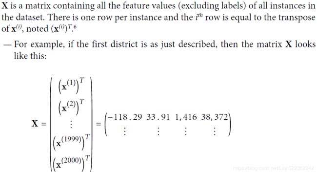
m is the number of instances in the dataset you are measuring the RMSE on.
![]() is a vector of all the feature values (excluding the label) of the
is a vector of all the feature values (excluding the label) of the ![]() instance in
instance in
the dataset, and ![]() is its label (the desired output value for that instance).
is its label (the desired output value for that instance).
—For example, if the first district in the dataset is located at longitude –118.29°,
latitude 33.91°, and it has 1,416 inhabitants with a median income of $38,372,
and the median house value is $156,400 (ignoring the other features for now),
then: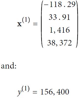
RMSE(X,h) is the cost function measured on the set of examples using your hypothesis h.
Even though the RMSE is generally the preferred performance measure for regression tasks, in some contexts you may prefer to use another function. For example, suppose that there are many outlier districts. In that case, you may consider using the Mean Absolute Error (also called the Average Absolute Deviation; see Equation 2-2):
Both the RMSE and the MAE are ways to measure the distance between two vectors: the vector of predictions and the vector of target values. Various distance measures, or norms, are possible:
* Computing the root of a sum of squares (RMSE) corresponds to the Euclidian norm: it is the notion of distance you are familiar with. It is also called the ℓ2 norm, noted ∥ · ∥2 (or just ∥ · ∥).
Computing the sum of absolutes (MAE) corresponds to the ℓ1 norm, noted ∥ · ∥1. It is sometimes called the Manhattan norm because it measures the distance between two points in a city if you can only travel along orthogonal city blocks.
The higher the norm index, the more it focuses on large values and neglects small ones. This is why the RMSE is more sensitive to outliers than the MAE. But when outliers are exponentially rare (like in a bell-shaped curve), the RMSE performs very well and is generally preferred.
Check the Assumptions
Lastly, it is good practice to list and verify the assumptions that were made so far (by you or others); this can catch serious issues early on. For example, the district prices that your system outputs are going to be fed into a downstream Machine Learning system, and we assume that these prices are going to be used as such. But what if the downstream system actually converts the prices into categories (e.g., “cheap,” “medium,” or “expensive”) and then uses those categories instead of the prices themselves? In this case, getting the price perfectly right is not important at all; your system
just needs to get the category right. If that’s so, then the problem should have been framed as a classification task, not a regression task. You don’t want to find this out after working on a regression system for months.
Fortunately, after talking with the team in charge of the downstream system, you are confident that they do indeed need the actual prices, not just categories. Great! You’re all set, the lights are green, and you can start coding now!
2. Get the Data and Download the Data
import os
import tarfile
from six.moves import urllib
DOWNLOAD_ROOT = 'https://raw.githubusercontent.com/ageron/handson-ml/master/'
HOUSING_URL = DOWNLOAD_ROOT + "datasets/housing/housing.tgz"
#or # os.path.abspath( os.path.join(os.getcwd(),'..') )
upperLevelDir=os.path.abspath( os.path.dirname(os.getcwd()) )
HOUSING_PATH = os.path.join(upperLevelDir,'datasets','housing')
HOUSING_PATH![]()
def fetch_housing_data(housing_url=HOUSING_URL, housing_path=HOUSING_PATH):
if not os.path.isdir(housing_path):
os.makedirs(housing_path) #creates a datasets/housing directory
tgz_path = os.path.join(housing_path, 'housing.tgz') #Storage path
urllib.request.urlretrieve(housing_url, tgz_path)
print(tgz_path)
housing_tgz = tarfile.open(tgz_path)
housing_tgz.extractall(path=housing_path) #extracts the housing.csv from it
housing_tgz.close()
#Now let’s load the data using Pandas
def load_housing_data(housing_path = HOUSING_PATH):
    csv_path = os.path.join(housing_path, 'housing.csv')
    return pd.read_csv(csv_path) #returns a Pandas DataFrame object containing all the data

fetch_housing_data()  #get csv file from housing.tgz


housing = load_housing_data()
housing.head() #Each row represents one district.
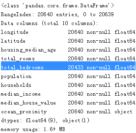
The info() method is useful to get a quick description of the data, in particular the total number of rows, and each attribute’s type and number of non-null values
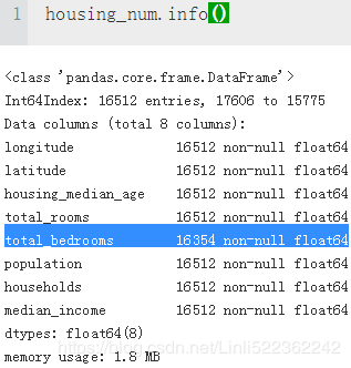
housing.info()There are 20,640 instances in the dataset, which means that it is fairly small by Machine Learning standards, but it’s perfect to get started. Notice that the total_bedrooms attribute has only 20,433 nonnull values, meaning that 207 districts are missing this feature. We will need to take care of this later
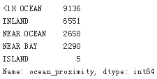
All attributes are numerical, except the ocean_proximity field. Its type is object, so it could hold any kind of Python object, but since you loaded this data from a CSV file you know that it must be a text attribute. When you looked at the top five rows, you probably noticed that the values in the ocean_proximity column were repetitive, which means that it is probably a categorical attribute. You can find out what categories exist and how many districts belong to each category by using the value_counts() method:
housing['ocean_proximity'].value_counts()housing.describe() #ignore categorical attributeThe count, mean, min, and max rows are self-explanatory. Note that the null values are ignored (so, for example, count of total_bedrooms is 20,433, not 20,640). The std row shows the standard deviation, which measures how dispersed the values are. The 25%, 50%, and 75% rows show the corresponding percentiles: a percentile indicates the value below which a given percentage of observations in a group of observations falls. For example, 25% of the districts have a housing_median_age lower than 18, while 50% are lower than 29 and 75% are lower than 37. These are often called the 25th percentile (or 1st quartile), the median, and the 75th percentile (or 3rd quartile).
Another quick way to get a feel of the type of data you are dealing with is to plot a histogram for each numerical attribute. A histogram shows the number of instances (on the vertical axis) that have a given value range (on the horizontal axis). You can either plot this one attribute at a time, or you can call the hist() method on the whole dataset, and it will plot a histogram for each numerical attribute (see Figure). For example, you can see that slightly over 800 districts have a median_house_value equal to about $100,000.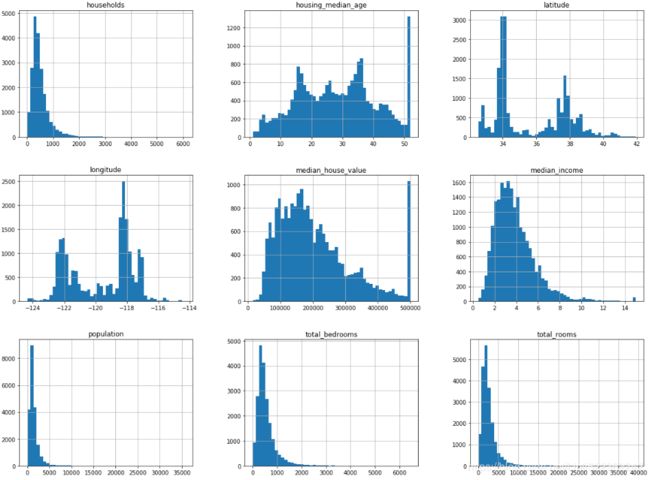
The hist() method relies on Matplotlib, which in turn relies on a user-specified graphical backend to draw on your screen. So before you can plot anything, you need to specify which backend Matplotlib should use. The simplest option is to use Jupyter’s magic command %matplotlib inline. This tells Jupyter to set up Matplotlib so it uses Jupyter’s own backend. Plots are then rendered within the notebook itself. Note that calling show() is optional in a Jupyter notebook, as Jupyter will automatically display plots when a cell is executed.
Notice a few things in these histograms:
1. First, the median income attribute does not look like it is expressed in US dollars (USD). After checking with the team that collected the data, you are told that the data has been scaled and capped
at 15 (actually 15.0001) for higher median incomes, and at 0.5 (actually 0.4999) for lower median
incomes. Working with preprocessed attributes is common in Machine Learning, and it is not
necessarily a problem, but you should try to understand how the data was computed.
2. The housing median age and the median house value were also capped被设了上限. The latter may be a serious
problem since it is your target attribute (your labels). Your Machine Learning algorithms may learn
that prices never go beyond that limit. You need to check with your client team (the team that will use
your system’s output) to see if this is a problem or not. If they tell you that they need precise
predictions even beyond $500,000, then you have mainly two options:
- a. Collect proper labels for the districts whose labels were capped.
- b. Remove those districts from the training set (and also from the test set, since your system should not be evaluated poorly if it predicts values beyond $500,000).
3. These attributes have very different scales. We will discuss this later in this chapter when we
explore feature scaling.
4. Finally, many histograms are tail heavy: they extend much farther to the right of the median than to
the left. This may make it a bit harder for some Machine Learning algorithms to detect patterns. We
will try transforming these attributes later on to have more bell-shaped distributions.
WARNING
Wait! Before you look at the data any further, you need to create a test set, put it aside, and never look at it.
Create a Test Set
It may sound strange to voluntarily set aside part of the data at this stage. After all, you have only taken a quick glance at the data, and surely you should learn a whole lot more about it before you decide what algorithms to use, right? This is true, but
your brain is an amazing pattern detection system, which means that it is highly prone to overfitting: if you look at the test set, you may stumble upon some seemingly interesting pattern in the test data that leads you to select a particular kind of
Machine Learning model. When you estimate the generalization error using the test set, your estimate will be too optimistic and you will launch a system that will not perform as well as expected. This is called data snooping bias.
Creating a test set is theoretically quite simple: just pick some instances randomly, typically 20% of the dataset, and set them aside:
import numpy as np

def split_train_test(data, test_ratio):
   #np.random.seed(42)
    shuffled_indices = np.random.permutation( len(data) )
    test_set_size = int( len(data)*test_ratio )
    test_indices = shuffled_indices[:test_set_size]
    train_indices = shuffled_indices[test_set_size:]
    return data.iloc[train_indices], data.iloc[test_indices]

train_set, test_set = split_train_test(housing, 0.2)
print(len(train_set), "train +", len(test_set), "test")![]()
Well, this works, but it is not perfect: if you run the program again, it will generate a different test set! Over time, you (or your Machine Learning algorithms) will get to see the whole dataset, which is what you want to avoid.
One solution is to save the test set on the first run and then load it in subsequent runs. Another option is to set the random number generator’s seed (e.g., np.random.seed(42)) before calling np.random.permutation(), so that it always generates the same shuffled indices.
But both these solutions will break next time you fetch an updated dataset. A common solution is to use
each instance’s identifier to decide whether or not it should go in the test set (assuming instances have a
unique and immutable identifier). For example, you could compute a hash of each instance’s identifier,
keep only the last byte of the hash, and put the instance in the test set if this value is lower or equal to 51
(~20% of 256). This ensures that the test set will remain consistent across multiple runs, even if you
refresh the dataset. The new test set will contain 20% of the new instances, but it will not contain any
instance that was previously in the training set. Here is a possible implementation:
def test_set_check(identifier, test_ratio, hash):
          #hash():compute a hash(bits) of identifier  #[-1]:the last byte of the hash,
          #The digest(bytes) is the output of the hash function. #2^8=256
    return hash(np.int64(identifier)).digest()[-1]<256 * test_ratio #contain 20% of the new instances

def split_train_test_by_id(data, test_ratio, id_column, hash=hashlib.md5):
    ids = data[id_column]
    in_test_set = ids.apply(lambda id_: test_set_check(id_, test_ratio, hash))
    return data.loc[~in_test_set], data.loc[in_test_set]
Unfortunately, the housing dataset does not have an identifier column. The simplest
solution is to use the row index as the ID:
housing_with_id = housing.reset_index() #add an 'index' column
train_set, test_set = split_train_test_by_id(housing_with_id, 0.2, 'index',)
train_set.head()
If you use the row index as a unique identifier, you need to make sure that new data gets appended to the end of the dataset, and no row ever gets deleted. If this is not possible, then you can try to use the most stable features to build a unique identifier.
For example, a district’s latitude and longitude are guaranteed to be stable for a few million years, so you could combine them into an ID like so:
housing_with_id['id'] = housing['longitude'] * 1000 + housing['latitude']
train_set, test_set = split_train_test_by_id(housing_with_id, 0.2, 'id')
train_set.head()
Scikit-Learn provides a few functions to split datasets into multiple subsets in various ways. The simplest function is train_test_split, which does pretty much the same thing as the function split_train_test defined earlier, with a couple of additional features. First there is a random_state parameter that allows you to set the random generator seed as explained previously, and second you can pass it multiple datasets with an identical number of rows, and it will split them on the same indices (this is very useful, for example, if you have a separate DataFrame for labels):
from sklearn.model_selection import train_test_split

train_set, test_set = train_test_split(housing, test_size=0.2, random_state=42)
train_set.head()
So far we have considered purely random sampling methods. This is generally fine if your dataset is large enough (especially relative to the number of attributes), but if it is not, you run the risk of introducing a significant sampling bias. When a survey company decides to call 1,000 people to ask them a few questions, they don’t just pick 1,000 people randomly in a phone booth. They try to ensure that these 1,000 people are representative of the whole population. For example, the US population is composed of 51.3% female and 48.7% male, so a well-conducted survey in the US would try to maintain this ratio in the sample: 513 female and 487 male. This is called stratified sampling: the population is divided into homogeneous subgroups called strata, and the right number of instances is sampled from each stratum to guarantee that the test set is representative of the overall population. If they used purely random sampling, there would be about 12% chance of sampling a skewed test set with either less than 49% female or more than 54% female. Either way, the survey results would be significantly biased.
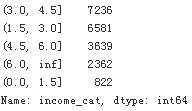
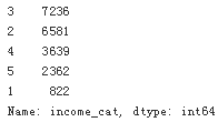
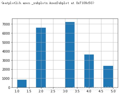
Suppose you chatted with experts who told you that the median income is a very important attribute to predict median housing prices. You may want to ensure that the test set is representative of the various categories of incomes in the whole dataset. Since the median income is a continuous numerical attribute, you first need to create an income category attribute. Let’s look at the median income histogram more closely (see Figure
housing['median_income'].hist() #a continuous numerical attribute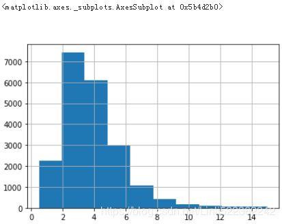
housing['income_cat'] = pd.cut(housing['median_income'],
                               bins=[0., 1.5, 3.0, 4.5, 6., np.inf],
                               #labels=[1,2,3,4,5]
                              )
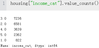
housing['income_cat'].value_counts()
housing['income_cat'] = pd.cut(housing['median_income'],
bins=[0., 1.5, 3.0, 4.5, 6., np.inf],
labels=[1,2,3,4,5]
)
housing['income_cat'].value_counts()housing["income_cat"].hist()(label 2-5 represents 1.5-6 tens of thousands of dollars)
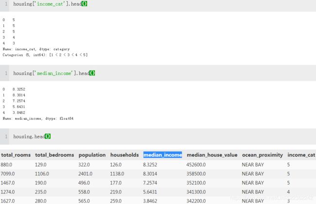
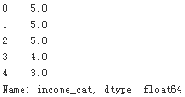
Most median income values are clustered around 1.5–6 (tens of thousands of dollars), but some median incomes go far beyond 6. It is important to have a sufficient number of instances in your dataset for each stratum, or else the estimate of the stratum’s importance may be biased. This means that you should not have too many strata, and each stratum should be large enough. The following code creates an income category attribute by dividing the median income by 1.5 (to limit the number of income categories), and rounding up using ceil (to have discrete categories), and then merging all the categories greater than 5 into category 5:
housing['income_cat'] = np.ceil(housing['median_income']/1.5)
#np.where( housing['income_cat']<5, housing['income_cat'], 5.0, inplace=True)
housing['income_cat'].where(housing['income_cat']<5, 5.0, inplace=True)
housing['income_cat'].head()
Now you are ready to do stratified sampling based on the income category. For this you can use Scikit-Learn’s StratifiedShuffleSplit class:
from sklearn.model_selection import StratifiedShuffleSplit

                              #n_splits: n groups of train/test pair
split = StratifiedShuffleSplit(n_splits=1, test_size=0.2, random_state=42) #one group of train/test pair
for train_index, test_index in split.split(housing, housing['income_cat']):
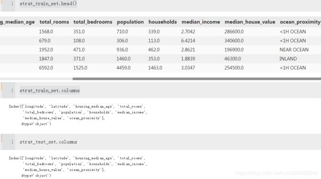
    strat_train_set = housing.loc[train_index]
    strat_test_set = housing.loc[test_index]
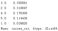
Let’s see if this worked as expected. You can start by looking at the income category proportions in the full housing dataset:
housing["income_cat"].value_counts() / len(housing) #len(housing): 20640
With similar code you can measure the income category proportions in the test set.
The following table compares the income category proportions in the overall dataset, in the test set generated with stratified sampling, and in a test set generated using purely random sampling. As you can see, the test set generated using stratified sampling has income category proportions almost identical to those in the full dataset, whereas the
test set generated using purely random sampling is quite skewed.
############Sampling bias comparison of stratified versus purely random sampling############
def income_cat_proportions(data):
    return data["income_cat"].value_counts() / len(data)

#purely random sampling
train_set, test_set = train_test_split(housing, test_size=0.2, random_state=42)

compare_props = pd.DataFrame({
    "Overall": income_cat_proportions(housing),
    "Stratified": income_cat_proportions(strat_test_set),
    "Random": income_cat_proportions(test_set),
}).sort_index() #strat_test_set["income_cat"]         #same label
compare_props["Random. %error"] = 100*compare_props["Random"] / compare_props["Overall"] -100
compare_props["Stratified. %error"] = 100*compare_props["Stratified"] / compare_props["Overall"] -100
compare_props
Now you should remove the income_cat attribute so the data is back to its original state:
for set in (strat_train_set, strat_test_set):
    set.drop(["income_cat"], axis=1, inplace=True)
We spent quite a bit of time on test set generation for a good reason: this is an often neglected but critical part of a Machine Learning project. Moreover, many of these ideas will be useful later when we discuss cross-validation. Now it’s time to move on to the next stage: exploring the data.
3.Discover and Visualize the Data to Gain Insights
So far you have only taken a quick glance at the data to get a general understanding of the kind of data you are manipulating. Now the goal is to go a little bit more in depth.
First, make sure you have put the test set aside and you are only exploring the training set. Also, if the training set is very large, you may want to sample an exploration set, to make manipulations easy and fast. In our case, the set is quite small so you can just work directly on the full set. Let’s create a copy so you can play with it without harming the training set:
housing = strat_train_set.copy() #deep copy #https://blog.csdn.net/u010712012/article/details/79754132
#https://blog.csdn.net/weixin_37275456/article/details/83033528 #df.copy(deep=True) is different with #copy.deepcopy(data)
Visualizing Geographical Data
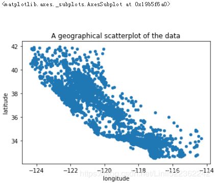
Since there is geographical information (latitude and longitude), it is a good idea to create a scatterplot of all districts to visualize the data
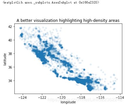
housing.plot(kind="scatter", x="longitude", y="latitude", title="A geographical scatterplot of the data")This looks like California all right, but other than that it is hard to see any particular pattern. Setting the alpha option to 0.1 makes it much easier to visualize the places where there is a high density of data points
housing.plot(kind="scatter", x="longitude", y="latitude", alpha=0.1,
             title="A better visualization highlighting high-density areas")
Now that’s much better: you can clearly see the high-density areas, namely the Bay
Area and around Los Angeles and San Diego, plus a long line of fairly high density in
the Central Valley, in particular around Sacramento and Fresno.
More generally, our brains are very good at spotting patterns图片中的规律 on pictures, but you
may need to play around with调整 visualization parameters to make the patterns stand
out.
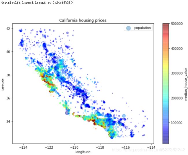
Now let’s look at the housing prices (Figure). The radius of each circle represents the district’s population (option s), and the color represents the price (option c). We will use a predefined color map (option cmap) called jet, which ranges from blue
(low values) to red (high prices):
housing.plot(kind="scatter", x="longitude", y="latitude", alpha=0.4,figsize=(10,7),
s=housing['population']/100, label="population",
c="median_house_value", cmap=plt.get_cmap("jet"), colorbar=True, sharex=False,
title="California housing prices"
)
plt.legend()
This image tells you that the housing prices are very much related to the location (e.g., close to the ocean) and to the population density, as you probably knew already. It will probably be useful to use a clustering algorithm to detect the main clusters, and add new features that measure the proximity接近度 to the cluster centers. The ocean proximity接近度 attribute may be useful as well, although in Northern California the housing prices in coastal districts are not too high, so it is not a simple rule.
Looking for Correlations
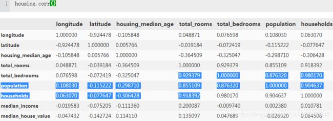
Since the dataset is not too large, you can easily compute the standard correlation coefficient (also called Pearson’s r) between every pair of attributes using the corr() method:
corr_matrix = housing.corr()
corr_matrix["median_house_value"].sort_values(ascending=False)
The correlation coefficient ranges from –1 to 1. When it is close to 1, it means that there is a strong positive correlation; for example, the median house value tends to go up when the median income goes up. When the coefficient is close to –1, it means that there is a strong negative correlation; you can see a small negative correlation
between the latitude and the median house value (i.e., prices have a slight tendency to
go down when you go north). Finally, coefficients close to zero mean that there is no
linear correlation.
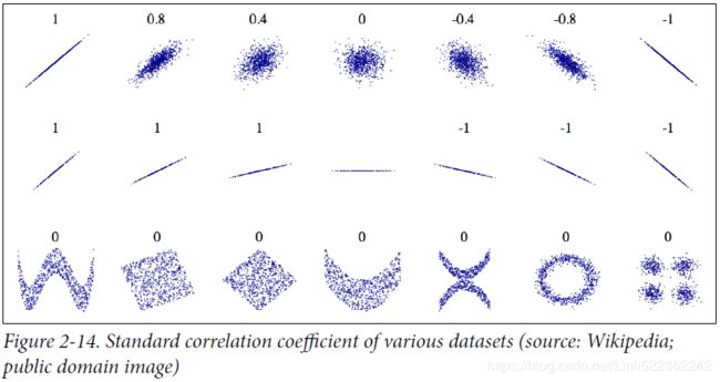
Figure 2-14 shows various plots along with the correlation coefficient between their horizontal and vertical axes.
The correlation coefficient only measures linear correlations (“if x goes up, then y generally goes up/down”). It may completely miss out on nonlinear relationships (e.g., “if x is close to zero then y generally goes up”). Note how all the plots of the bottom row have a correlation coefficient equal to zero despite the fact that their axes are clearly not independent: these are examples of nonlinear relationships. Also, the second row shows examples where the correlation
coefficient is equal to 1 or –1; notice that this has nothing to do with the slope. For example, your height in inches has a correlation coefficient of 1 with your height in feet or in nanometers.
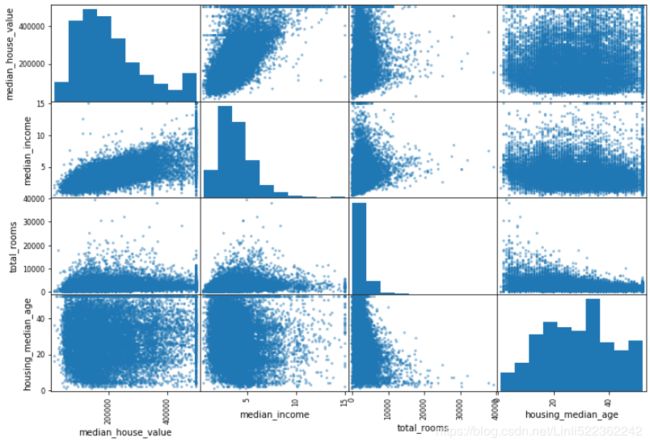
Another way to check for correlation between attributes is to use Pandas’ scatter_matrix function, which plots every numerical attribute against every other numerical attribute. Since there are now 11 numerical attributes, you would get 11^2 = 121 plots, which would not fit on a page, so let’s just focus on a few promising attributes that seem most correlated with the median housing value (Figure):
from pandas.plotting import scatter_matrix
attributes = ["median_house_value", "median_income", "total_rooms", "housing_median_age"]
scatter_matrix(housing[attributes], figsize=(12,8))
plt.show()
The main diagonal (top left to bottom right) would be full of straight lines if Pandas plotted each variable against itself, which would not be very useful. So instead Pandas displays a histogram of each attribute(frequency) (other options are available; see Pandas’ documentation for more details).
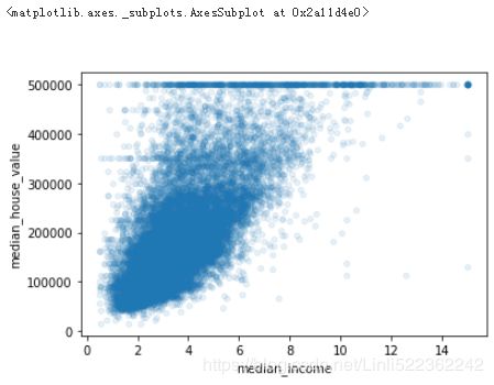
The most promising最有希望的 attribute to predict the median house value is the median income, so let’s zoom in放大 on their correlation scatterplot (Figure)
housing.plot(kind="scatter", x="median_income", y="median_house_value", alpha=0.1)
This plot reveals a few things. First, the correlation is indeed very strong; you can clearly see the upward trend and the points are not too dispersed. Second, the price cap that we noticed earlier is clearly visible as a horizontal line at 500,000.But this plot reveals other less obvious straight lines: a horizontal line around $450,000, another around $350,000, perhaps one around $280,000, and a few more below that. You may want to try removing the corresponding districts to prevent your algorithms from learning to reproduce these data quirks巧合.
Experimenting with Attribute Combinations
Hopefully the previous sections gave you an idea of a few ways you can explore the data and gain insights. You identified a few data quirks that you may want to clean up before feeding the data to a Machine Learning algorithm, and you found interesting correlations between attributes, in particular with the target attribute. You also noticed that some attributes have a tail-heavy distribution, so you may want to transform them (e.g., by computing their logarithm). Of course, your mileage will vary considerably with each project, but the general ideas are similar.
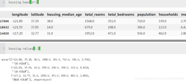
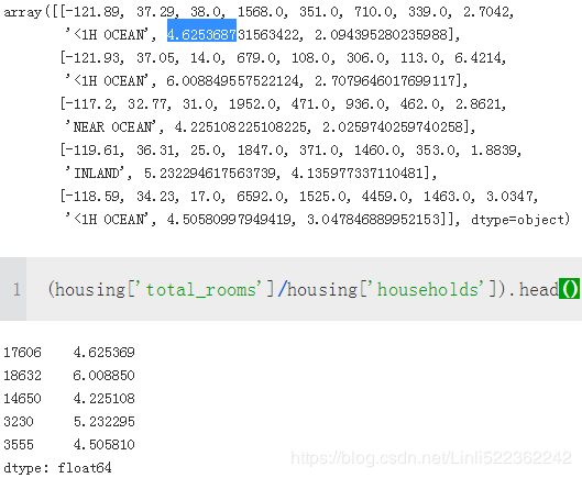
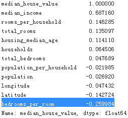
One last thing you may want to do before actually preparing the data for Machine Learning algorithms is to try out various attribute combinations. For example, the total number of rooms in a district is not very useful if you don’t know how many households there are. What you really want is the number of rooms per household. Similarly, the total number of bedrooms by itself is not very useful: you probably want to compare it to the number of rooms. And the population per household also seems like an interesting attribute combination to look at. Let’s create these new attributes:
housing['rooms_per_household'] = housing["total_rooms"]/housing["households"]
housing["bedrooms_per_room"] = housing["total_bedrooms"]/housing["total_rooms"]
housing["population_per_household"] = housing["population"]/housing["households"]

corr_matrix=housing.corr()
corr_matrix["median_house_value"].sort_values(ascending=False)
Hey, not bad! The new bedrooms_per_room attribute is much more correlated with the median house value than the total number of rooms or bedrooms. Apparently houses with a lower bedroom/room ratio tend to be more expensive. The number of rooms per household is also more informative than the total number of rooms in a district—obviously the larger the houses, the more expensive they are.
This round of exploration does not have to be absolutely thorough; the point is to start off on the right foot and quickly gain insights that will help you get a first reasonably good prototype. But this is an iterative process: once you get a prototype up and running, you can analyze its output to gain more insights and come back to this exploration step.
4.Prepare the Data for Machine Learning Algorithms
It’s time to prepare the data for your Machine Learning algorithms. Instead of just doing this manually, you should write functions to do that, for several good reasons:
• This will allow you to reproduce these transformations easily on any dataset (e.g., the next time you get a fresh dataset).
• You will gradually build a library of transformation functions that you can reuse in future projects.
• You can use these functions in your live system to transform the new data before feeding it to your algorithms.
• This will make it possible for you to easily try various transformations and see which combination of transformations works best.
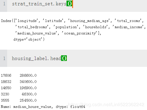
But first let’s revert to a clean training set (by copying strat_train_set once again), and let’s separate the predictors and the labels since we don’t necessarily want to apply the same transformations to the predictors and the target values (note that drop() creates a copy of the data and does not affect strat_train_set):
housing = strat_train_set.drop('median_house_value', axis=1)  #return a dataframe without the dropped column
housing_label = strat_train_set["median_house_value"].copy()
housing.keys()
Data Cleaning
Most Machine Learning algorithms cannot work with missing features, so let’s create
a few functions to take care of them. You noticed earlier that the total_bedrooms
attribute has some missing values, so let’s fix this. You have three options:
• Get rid of the corresponding districts.
• Get rid of the whole attribute.
• Set the values to some value (zero, the mean, the median, etc.).
You can accomplish these easily using DataFrame’s dropna(), drop(), and fillna()
methods:
housing.dropna(subset=["total_bedrooms"]) # option 1
housing.drop("total_bedrooms", axis=1) # option 2
median = housing["total_bedrooms"].median()
housing["total_bedrooms"].fillna(median) # option 3
If you choose option 3, you should compute the median value on the training set, and use it to fill the missing values in the training set, but also don’t forget to save the median value that you have computed. You will need it later to replace missing values in the test set when you want to evaluate your system, and also once the system goes live to replace missing values in new data.
Scikit-Learn provides a handy class to take care of missing values: Imputer. Here is how to use it. First, you need to create an Imputer instance, specifying that you want to replace each attribute’s missing values with the median of that attribute:
#pip install --user --upgrade scikit-learn==0.19.1
from sklearn.preprocessing import Imputer
imputer = Imputer(strategy="median") #estimator’s hyperparameters
Since the median can only be computed on numerical attributes, we need to create a copy of the data without the text attribute ocean_proximity:
housing_num = housing.drop("ocean_proximity", axis=1)
Now you can fit the imputer instance to the training data using the fit() method:
imputer.fit(housing_num)![]()
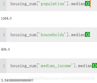
The imputer has simply computed the median of each attribute and stored the result in its statistics_ instance variable. Only the total_bedrooms attribute had missing values, but we cannot be sure that there won’t be any missing values in new data after the system goes live, so it is safer to apply the imputer to all the numerical attributes:
imputer.statistics_ #estimator’s learned parameters![]()
housing_num.median().values![]()
##################################################################
housing_num.loc[ (housing_num['longitude']==-118.51) & (housing_num['latitude']==34.26) ]
housing_num.loc[housing_num['longitude']==-118.51][housing_num['latitude']==34.26]
housing_num['total_rooms'].median() #ignore the missing value
![]()
housing_num['total_bedrooms'].median()
![]()
##################################################################
Now you can use this “trained” imputer to transform the training set by replacing missing values by the learned medians:
X = imputer.transform(housing_num) #Transform the training set
The result is a plain Numpy array containing the transformed features. If you want to put it back into a Pandas DataFrame, it’s simple:
housing_tr = pd.DataFrame(X, columns=housing_num.columns, index=housing.index)
housing_tr.describe() #will not change the dataset's describtion if compare it with original dataset's describtion
sample_incomplete_rows = housing[ housing.isnull().any(axis=1) ].head()
sample_incomplete_rowshousing_tr.loc[sample_incomplete_rows.index.values]#########################################################################################
Scikit-Learn Design
Scikit-Learn’s API is remarkably well designed. The main design principles are:
- Consistency. All objects share a consistent and simple interface:
- —Estimators. Any object that can estimate some parameters based on a dataset is called an estimator (e.g., an imputer is an estimator). The estimation itself is performed by the fit() method, and it takes only a dataset as a parameter (or two for supervised learning algorithms; the second dataset contains the labels). Any other parameter needed to guide the estimation process is considered a hyperparameter (such as an imputer’s strategy='median'), and it must be set as an instance variable (generally via a constructor parameter).
- —Transformers. Some estimators (such as an imputer) can also transform a dataset; these are called transformers. Once again, the API is quite simple: the transformation is performed by the transform() method with the dataset to transform as a parameter. It returns the transformed dataset. This transformation generally relies on the learned parameters, as is the case for an imputer. All transformers also have a convenience method called fit_transform() that is equivalent to calling fit() and then transform() (but sometimes fit_transform() is optimized and runs much faster).
- —Predictors. Finally, some estimators are capable of making predictions given a dataset; they are called predictors. For example, the LinearRegression model in the previous chapter was a predictor: it predicted life satisfaction given a country’s GDP per capita. A predictor has a predict() method that takes a dataset of new instances and returns a dataset of corresponding predictions. It also has a score() method that measures the quality of the predictions given a test set (and the corresponding labels in the case of supervised learning algorithms).
- Inspection. All the estimator’s hyperparameters are accessible directly via public instance variables (e.g., imputer.strategy), and all the estimator’s learned parameters are also accessible via public instance variables with an underscore suffix (e.g., imputer.statistics_).
- Nonproliferation of classes. Datasets are represented as NumPy arrays or SciPy sparse matrices, instead of homemade自制的 classes. Hyperparameters are just regular Python strings or numbers.
- Composition. Existing building blocks are reused as much as possible. For example, it is easy to create a Pipeline estimator from an arbitrary sequence of transformers followed by a final estimator, as we will see.
- Sensible合乎情理的 defaults. Scikit-Learn provides reasonable default values for most parameters, making it easy to create a baseline working system quickly.
#########################################################################################
Handling Text and Categorical Attributes
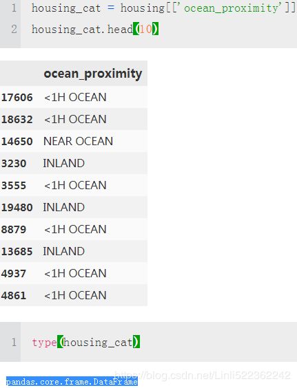
Earlier we left out the categorical attribute ocean_proximity because it is a text attribute so we cannot compute its median. Most Machine Learning algorithms prefer to work with numbers anyway, so let’s convert these text labels to numbers.
#Now let's preprocess the categorical input feature, ocean_proximity:
housing_cat = housing['ocean_proximity']
housing_cat_encoded, housing_categories = housing_cat.factorize()
housing_cat_encoded
![]()
housing_categories
![]()
one attribute equal to 1 when the category is “<1H OCEAN” (and 0 otherwise), another attribute equal to 1 when the category is “INLAND” (and 0 otherwise), and so on. This is called one-hot encoding, because only one attribute will be equal to 1 (hot), while the others will be 0 (cold).
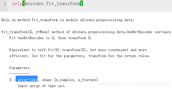
Scikit-Learn provides a OneHotEncoder encoder to convert integer categorical values into one-hot vectors. Let’s encode the categories as one-hot vectors. Note that fit_transform() expects a 2D array, but housing_cat_encoded is a 1D array, so we need to reshape it
from sklearn.preprocessing import OneHotEncoder
encoder = OneHotEncoder()
housing_cat_1hot = encoder.fit_transform(housing_cat_encoded.reshape(-1,1)) #reshape(-1,1): one column of 2D arr
housing_cat_1hot![]()
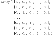
Notice that the output is a SciPy sparse matrix, instead of a NumPy array. This is very useful when you have categorical attributes with thousands of categories. After onehot encoding we get a matrix with thousands of columns, and the matrix is full of zeros except for one 1 per row. Using up tons of memory mostly to store zeros would be very wasteful, so instead a sparse matrix only stores the location of the nonzero elements. You can use it mostly like a normal 2D array,19 but if you really want to convert it to a (dense) NumPy array, just call the toarray() method:
housing_cat_1hot.toarray() #'<1H OCEAN', 'NEAR OCEAN', 'INLAND', 'NEAR BAY', 'ISLAND' #if exists columname
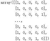
We can apply both transformations (from text categories to integer categories, then from integer categories to one-hot vectors) in one shot using the LabelBinarizer class:
from sklearn.preprocessing import LabelBinarizer

encoder = LabelBinarizer()
housing_cat_1hot = encoder.fit_transform(housing_cat)
housing_cat_1hot
#since my Anaconda cannot install CategoricalEncoder, I have to use CategoricalEncoder Class
from sklearn.base import BaseEstimator, TransformerMixin
from sklearn.utils import check_array
from sklearn.preprocessing import LabelEncoder
from scipy import sparse

class CategoricalEncoder(BaseEstimator, TransformerMixin):
    def __init__(self, encoding='onehot', categories='auto', dtype=np.float64, handle_unknown='error'):
        self.encoding = encoding
        self.categories = categories
        self.dtype = dtype
        self.handle_unknown = handle_unknown

    def fit(self, X, y=None):
        """Fit the CategoricalEncoder to X.
        Parameters
        ----------
        X : array-like, shape [n_samples, n_feature]
        The data to determine the categories of each feature.
        Returns
        -------
        self
        """
        if self.encoding not in ['onehot', 'onehot-dense', 'ordinal']:
            template = ("encoding should be either 'onehot', 'onehot-dense' or 'ordinal', got %s")
            raise ValueError(template % self.handle_unknown)

        if self.handle_unknown not in ['error', 'ignore']:
            template = ("handle_unknown should be either 'error' or 'ignore', got %s")
            raise ValueError(template % self.handle_unknown)

        if self.encoding == 'ordinal' and self.handle_unknown == 'ignore':
            raise ValueError("handle_unknown='ignore' is not supported for encoding='ordinal'")

        #check_array: By default, the input(here is X) is converted to an at least 2D numpy array.
        #If the dtype of the array is object, attempt converting to float, raising on failure.
        #csc_matrix: https://docs.scipy.org/doc/scipy/reference/generated/scipy.sparse.csc_matrix.html
        X = check_array(X, dtype=np.object, accept_sparse='csc', copy=True)
        n_samples, n_features = X.shape   #(16512, 1)

        #the prefix underscore: private variable,
        #the trailing underscore is used by convention to avoid naming conflicts
        self._label_encoders_ = [LabelEncoder() for _ in range(n_features)]    #[LabelEncoder, ...]
        for i in range(n_features):
            le = self._label_encoders_[i]
            Xi = X[:, i]
            if self.categories == 'auto':
                le.fit(Xi)
            else:
                #np.in1d(ar1,ar2): Returns a boolean array the same length as ar1 that
                #is True where an element of ar1 is in ar2
                #and False otherwise.
                valid_mask = np.in1d(Xi, self.categories[i])
                if not np.all(valid_mask):
                    if self.handle_unknown == 'error':
                        diff = np.unique(Xi[~valid_mask])
                        msg = ("Found unknown categories {0} in column {1} during fit".format(diff, i))
                        raise ValueError(msg)
                le.classes_ = np.array(np.sort(self.categories[i]))
        #for examples,here is ['<1H OCEAN' 'INLAND' 'ISLAND' 'NEAR BAY' 'NEAR OCEAN']
        #encoder.classes_
        self.categories_ = [le.classes_ for le in self._label_encoders_]
        return self

    def transform(self, X):
        """Transform X using one-hot encoding.
        Parameters
        ----------
        X : array-like, shape [n_samples, n_features]
        The data to encode.
        Returns
        -------
        X_out : sparse matrix or a 2-d array
        Transformed input.
        """
        #check_array: By default, the input(here is X) is converted to an at least 2D numpy array.
        #If the dtype of the array is object, attempt converting to float, raising on failure.
        #csc_matrix: https://docs.scipy.org/doc/scipy/reference/generated/scipy.sparse.csc_matrix.html
        X = check_array(X, accept_sparse='csc', dtype=np.object, copy=True)
        n_samples, n_features = X.shape
        X_int = np.zeros_like(X, dtype=np.int)
        X_mask = np.ones_like(X, dtype=np.bool) #dtype:Overrides the data type of the result
                                                #conver the 1s to all True

        for i in range(n_features):
            #Returns a boolean array the same length as ar1 that is True where an element of ar1 is in ar2
            #and False otherwise.
            valid_mask = np.in1d(X[:, i], self.categories_[i]) #[ True  True  True ...  True  True  True]

            if not np.all(valid_mask):
                if self.handle_unknown == 'error':
                    diff = np.unique(X[~valid_mask, i])
                    msg = ("Found unknown categories {0} in column {1} during transform".format(diff, i))
                    raise ValueError(msg)
                else:
                    # Set the problematic rows to an acceptable value and
                    # continue `The rows are marked `X_mask` and will be
                    # removed later.
                    X_mask[:, i] = valid_mask
                    X[:, i][~valid_mask] = self.categories_[i][0]
            X_int[:, i] = self._label_encoders_[i].transform(X[:, i])  #[0 0 4 ... 1 0 3]  here only one column #len(row_indices)

            if self.encoding == 'ordinal':
                return X_int.astype(self.dtype, copy=False)
            mask = X_mask.ravel() #[ True  True  True ...  True  True  True]
           #self.categories_: [array(['<1H OCEAN', 'INLAND', 'ISLAND', 'NEAR BAY', 'NEAR OCEAN'], dtype=object)]
           #cats.shape[0]: 5
            n_values = [cats.shape[0] for cats in self.categories_] #[[5]]
            n_values = np.array([0] + n_values)   #np.array( [[0] [5]] )
            indices = np.cumsum(n_values)   #[0 5]  #start with 0, size=5 columns


            #X_int:  2D numpy array, here only one column
            #indices[:-1] : [0]
            #X_int + indices[:-1]: #matrix plus#[ [0 0 4 ... 1 0 3]^T ]
            column_indices = (X_int + indices[:-1]).ravel()[mask]    #extraction: [0 0 4 ... 1 0 3]
            row_indices = np.repeat(np.arange(n_samples, dtype=np.int32),n_features)[mask]
            data = np.ones(n_samples * n_features)[mask]
            #csc_matrix: https://docs.scipy.org/doc/scipy/reference/generated/scipy.sparse.csc_matrix.html

                                                                 #position  #len(row_indices)==len(column_indices)
            out = sparse.csc_matrix((data, (row_indices, column_indices)),
                                     shape=(n_samples, indices[-1]),  #(16512,5)
                                     dtype=self.dtype
                                   ).tocsr()
            if self.encoding == 'onehot-dense':
                return out.toarray()
            else:
                return out

        Parameters
        ----------
        X : array-like, shape [n_samples, n_feature]
        The data to determine the categories of each feature.
        Returns
        -------
        self
        """
        if self.encoding not in ['onehot', 'onehot-dense', 'ordinal']:
            template = ("encoding should be either 'onehot', 'onehot-dense' or 'ordinal', got %s")
            raise ValueError(template % self.handle_unknown)

        if self.handle_unknown not in ['error', 'ignore']:
            template = ("handle_unknown should be either 'error' or 'ignore', got %s")
            raise ValueError(template % self.handle_unknown)

        if self.encoding == 'ordinal' and self.handle_unknown == 'ignore':
            raise ValueError("handle_unknown='ignore' is not supported for encoding='ordinal'")
        X = check_array(X, dtype=np.object, accept_sparse='csc', copy=True)
        n_samples, n_features = X.shape

        self._label_encoders_ = [LabelEncoder() for _ in range(n_features)]
        for i in range(n_features):
            le = self._label_encoders_[i]
            Xi = X[:, i]
            if self.categories == 'auto':
                le.fit(Xi)
            else:
                valid_mask = np.in1d(Xi, self.categories[i])
                if not np.all(valid_mask):
                    if self.handle_unknown == 'error':
                        diff = np.unique(Xi[~valid_mask])
                        msg = ("Found unknown categories {0} in column {1} during fit".format(diff, i))
                        raise ValueError(msg)
                le.classes_ = np.array(np.sort(self.categories[i]))
        self.categories_ = [le.classes_ for le in self._label_encoders_]
        return self

    def transform(self, X):
        """Transform X using one-hot encoding.
        Parameters
        ----------
        X : array-like, shape [n_samples, n_features]
        The data to encode.
        Returns
        -------
        X_out : sparse matrix or a 2-d array
        Transformed input.
        """
        X = check_array(X, accept_sparse='csc', dtype=np.object, copy=True)
        n_samples, n_features = X.shape
        X_int = np.zeros_like(X, dtype=np.int)
        X_mask = np.ones_like(X, dtype=np.bool)

        for i in range(n_features):
            valid_mask = np.in1d(X[:, i], self.categories_[i])

            if not np.all(valid_mask):
                if self.handle_unknown == 'error':
                    diff = np.unique(X[~valid_mask, i])
                    msg = ("Found unknown categories {0} in column {1} during transform".format(diff, i))
                    raise ValueError(msg)
                else:
                    # Set the problematic rows to an acceptable value and
                    # continue `The rows are marked `X_mask` and will be
                    # removed later.
                    X_mask[:, i] = valid_mask
                    X[:, i][~valid_mask] = self.categories_[i][0]
            X_int[:, i] = self._label_encoders_[i].transform(X[:, i])

            if self.encoding == 'ordinal':
                return X_int.astype(self.dtype, copy=False)
            mask = X_mask.ravel()
            n_values = [cats.shape[0] for cats in self.categories_]
            n_values = np.array([0] + n_values)
            indices = np.cumsum(n_values)

            column_indices = (X_int + indices[:-1]).ravel()[mask]
            row_indices = np.repeat(np.arange(n_samples, dtype=np.int32),n_features)[mask]
            data = np.ones(n_samples * n_features)[mask]

            out = sparse.csc_matrix((data, (row_indices, column_indices)),
                                    shape=(n_samples, indices[-1]),
                                    dtype=self.dtype).tocsr()
            if self.encoding == 'onehot-dense':
                return out.toarray()
            else:
                return out

#from sklearn.preprocessing import CategoricalEncoder # in future versions of Scikit-Learn
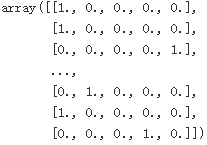
cat_encoder = CategoricalEncoder()
housing_cat_reshaped = housing_cat.values.reshape(-1,1)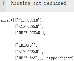
housing_cat_1hot = cat_encoder.fit_transform(housing_cat_reshaped)
housing_cat_1hot.toarray()
Custom Transformers
Although Scikit-Learn provides many useful transformers, you will need to write your own for tasks such as custom cleanup operations or combining specific attributes. You will want your transformer to work seamlessly with Scikit-Learn functionalities (such as pipelines), and since Scikit-Learn relies on duck typing (not inheritance), all you need is to create a class and implement three methods: fit() (returning self), transform(), and fit_transform(). You can get the last one for
free by simply adding TransformerMixin as a base class. Also, if you add BaseEstimator as a base class (and avoid *args and **kargs in your constructor) you will get two extra methods (get_params() and set_params()) that will be useful for automatic hyperparameter tuning. For example, here is a small transformer class that adds the combined attributes we discussed earlier: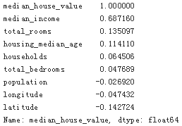
from sklearn.base import BaseEstimator, TransformerMixin
rooms_ix, bedrooms_ix, population_ix, household_ix = 3,4,5,6

class CombinedAttributesAdder(BaseEstimator, TransformerMixin):
    def __init__(self, add_bedrooms_per_room = True): #no *args or **kargs
        self.add_bedrooms_per_room = add_bedrooms_per_room
    def fit(self, X, y=None):
        return self #nothing else to do
    def transform(self, X, y=None):
        rooms_per_household = X[:, rooms_ix] / X[:, household_ix]
        population_per_household = X[:, population_ix] / X[:, household_ix]

        if self.add_bedrooms_per_room:
            bedrooms_per_room = X[:, bedrooms_ix] / X[:,rooms_ix]
            #Translates slice objects to concatenation along the second axis.
            return np.c_[X, rooms_per_household, population_per_household, bedrooms_per_room]
        else:
            return np.c_[X, rooms_per_household, population_per_household]

attr_adder = CombinedAttributesAdder(add_bedrooms_per_room=False)
housing_extra_attribs = attr_adder.transform(housing.values)
housing_extra_attribs[:5]
In this example the transformer has one hyperparameter, add_bedrooms_per_room, set to True by default (it is often helpful to provide sensible defaults). This hyperparameter will allow you to easily find out whether adding this attribute helps the
Machine Learning algorithms or not. More generally, you can add a hyperparameter to gate any data preparation step that you are not 100% sure about. The more you automate these data preparation steps, the more combinations you can automatically try out, making it much more likely that you will find a great combination (and saving
you a lot of time).
Feature Scaling
One of the most important transformations you need to apply to your data is feature scaling. With few exceptions, Machine Learning algorithms don’t perform well when the input numerical attributes have very different scales. This is the case for the housing data: the total number of rooms ranges from about 6 to 39,320, while the median incomes only range from 0 to 15. Note that scaling the target values is generally not required.
There are two common ways to get all attributes to have the same scale: min-max scaling and standardization.
Min-max scaling (many people call this normalization) is quite simple: values are shifted and rescaled so that they end up ranging from 0 to 1. We do this by subtracting the min value and dividing by the max minus the min. Scikit-Learn provides a transformer called MinMaxScaler for this. It has a feature_range hyperparameter that lets you change the range if you don’t want 0–1 for some reason.
Standardization is quite different: first it subtracts the mean value (so standardized values always have a zero mean), and then it divides by the variance so that the resulting distribution has unit variance. Unlike min-max scaling, standardization does not bound values to a specific range, which may be a problem for some algorithms (e.g.,
neural networks often expect an input value ranging from 0 to 1). However, standardization is much less affected by outliers. For example, suppose a district had a median income equal to 100 (by mistake). Min-max scaling would then crush all the other values from 0–15 down to 0–0.15, whereas standardization would not be much affected.
Scikit-Learn provides a transformer called StandardScaler for standardization.
WARNING
As with all the transformations, it is important to fit the scalers to the training data only, not to the full dataset (including the test set). Only then can you use them to transform the training set and the test set (and new data).
Transformation Pipelines
As you can see, there are many data transformation steps that need to be executed in the right order. Fortunately, Scikit-Learn provides the Pipeline class to help with such sequences of transformations. Here is a small pipeline for the numerical attributes:
from sklearn.pipeline import Pipeline
from sklearn.preprocessing import StandardScaler
num_pipeline = Pipeline([
    ('imputer', Imputer(strategy="median")),
    ('attr_adder', CombinedAttributesAdder()),
    ('std_scaler', StandardScaler()), #must have a fit_transform() method since its output must be passed to pipeline
])
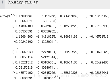
housing_num_tr = num_pipeline.fit_transform(housing_num)
Standardization is quite different: first it subtracts the mean value (so standardized values always have a zero mean), and then it divides by the variance so that the resulting distribution has unit variance.
The Pipeline constructor takes a list of name/estimator pairs defining a sequence of steps. All but the last estimator must be transformers (i.e., they must have a fit_transform() method). The names can be anything you like(as long as they don’t contain double underscores “__”)..
When you call the pipeline’s fit() method, it calls fit_transform() sequentially on all transformers, passing the output of each call as the parameter to the next call, until it reaches the final estimator, for which it just calls the fit() method.
The pipeline exposes the same methods as the final estimator. In this example, the last estimator is a StandardScaler, which is a transformer, so the pipeline has a transform() method that applies all the transforms to the data in sequence (it also has a fit_transform method that we could have used instead of calling fit() and then transform()).
Now it would be nice if we could feed a Pandas DataFrame directly into our pipeline, instead of having to first manually extract the numerical columns into a NumPy array. There is nothing in Scikit-Learn to handle Pandas DataFrames, but we can write a custom transformer for this task:
Each subpipeline starts with a selector transformer: it simply transforms the data by selecting the desired attributes (numerical or categorical), dropping the rest, and converting the resulting DataFrame to a NumPy array.
from sklearn.base import BaseEstimator, TransformerMixin

class DataFrameSelector(BaseEstimator, TransformerMixin):
    def __init__(self, attribute_names):
        self.attribute_names = attribute_names

    def fit(self, X, y=None):
        return self

    def transform(self, X):
        return X[self.attribute_names].values
Our DataFrameSelector will transform the data by selecting the desired attributes, dropping the rest, and converting the resulting DataFrame to a NumPy array. With this, you can easily write a pipeline that will take a Pandas DataFrame and handle only the numerical values: the pipeline would just start with a DataFrameSelector to pick only the numerical attributes, followed by the other preprocessing steps we discussed earlier. And you can just as easily write another pipeline for the categorical attributes as well by simply selecting the categorical attributes using a DataFrameSelector and then applying a LabelBinarizer .
You now have a pipeline for numerical values, and you also need to apply the LabelBinarizer on the categorical values: how can you join these transformations into a single pipeline? Scikit-Learn provides a FeatureUnion class for this. You give it a list of transformers (which can be entire transformer pipelines), and when its transform() method is called it runs each transformer’s transform() method in parallel, waits for their output, and then concatenates them and returns the result (and of course calling its fit() method calls all each transformer’s fit() method). A full pipeline handling both numerical and categorical attributes may look like this:
from sklearn.pipeline import FeatureUnion #Sckit-learn <0.20
from sklearn.pipeline import Pipeline
from sklearn.preprocessing import StandardScaler
housing_num = housing.drop('ocean_proximity', axis=1)#return a dataframe without the dropped column
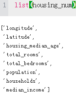
num_attribs = list(housing_num)
cat_attribs = ["ocean_proximity"]
num_pipeline=Pipeline([
('selector', DataFrameSelector(num_attribs)),
('imputer', Imputer(strategy='median')),
('attribs_adder', CombinedAttributesAdder()),
('std_scaler', StandardScaler()),
])
cat_pipeline = Pipeline([
('selector', DataFrameSelector(cat_attribs)),
('label_binarizer', CategoricalEncoder(encoding="onehot-dense"))
])
full_pipeline = FeatureUnion(n_jobs=1, #default 1
transformer_list=[('num_pipeline', num_pipeline),
('cat_pipeline', cat_pipeline),
]
)
housing_prepared = full_pipeline.fit_transform(housing)And you can run the whole pipeline simply:
housing_prepared = full_pipeline.fit_transform(housing)
housing_prepared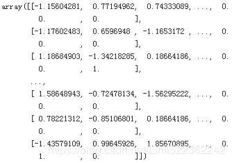
housing_prepared.shape![]()
#############################Scikit-learn >0.20
#https://github.com/ageron/handson-ml/blob/master/02_end_to_end_machine_learning_project.ipynb
#https://github.com/ageron/handson-ml2/blob/master/02_end_to_end_machine_learning_project.ipynb
from sklearn.compose import ColumnTransformer # Scikit-Learn > 0.20
from sklearn.pipeline import Pipeline
from sklearn.preprocessing import StandardScaler

num_attribs = list(housing_num)
cat_attribs = ["ocean_proximity"]

num_pipeline = Pipeline([
        ('imputer', SimpleImputer(strategy="median")),
        ('attribs_adder', CombinedAttributesAdder()),
        ('std_scaler', StandardScaler()),
    ])

cat_pipeline = Pipeline([
    ('cat_encoder', OneHotEncoder()),  # if error, instead CategoricalEncoder(encoding="onehot-dense")
])

full_pipeline = ColumnTransformer([
        ("num", num_pipeline, num_attribs),
        ("cat", cat_pipeline, cat_attribs),
    ])

housing_prepared = full_pipeline.fit_transform(housing)
housing_prepared = full_pipeline.fit_transform(housing)
housing_prepared
housing_prepared.shape![]()
#############################
02_End-to-End Machine Learning Project_02_stats.sem_Cross_Validation_Grid_Randomized_Ensemble_ Pipel
https://blog.csdn.net/Linli522362242/article/details/103587172
02_End-to-End Machine Learning Project_03_stats.sem_ppf_CategoricalEncoder_RandomizedSearchCV_joblib
https://blog.csdn.net/Linli522362242/article/details/103646927
