何宽

【中文】【吴恩达课后编程作业】Course 1 - 神经网络和深度学习 - 第四周作业(1&2)

【吴恩达课后编程作业】01 - 神经网络和深度学习 - 第四周 - PA1&2 - 一步步搭建多层神经网络以及应用

上一篇：【课程1 - 第四周测验】※※※※※ 【回到目录】※※※※※下一篇：【课程2 - 第一周测验】

声明

本文参考Kulbear 的【Building your Deep Neural Network - Step by Step】和【Deep Neural Network - Application】，以及念师的【8. 多层神经网络代码实战】，我基于以上的文章加以自己的理解发表这篇博客，力求让大家以最轻松的姿态理解吴恩达的视频，如有不妥的地方欢迎大家指正。

本文所使用的资料已上传到百度网盘【点击下载】，提取码：xx1w，请在开始之前下载好所需资料，或者在本文底部copy资料代码。

【博主使用的python版本：3.6.2】

开始之前

在正式开始之前，我们先来了解一下我们要做什么。在本次教程中，我们要构建两个神经网络，一个是构建两层的神经网络，一个是构建多层的神经网络，多层神经网络的层数可以自己定义。本次的教程的难度有所提升，但是我会力求深入简出。在这里，我们简单的讲一下难点，本文会提到**[LINEAR-> ACTIVATION]转发函数，比如我有一个多层的神经网络，结构是输入层->隐藏层->隐藏层->···->隐藏层->输出层**，在每一层中，我会首先计算Z = np.dot(W,A) + b，这叫做【linear_forward】，然后再计算A = relu(Z) 或者 A = sigmoid(Z)，这叫做【linear_activation_forward】，合并起来就是这一层的计算方法，所以每一层的计算都有两个步骤，先是计算Z，再计算A，你也可以参照下图：

我们来说一下步骤：

初始化网络参数
前向传播

2.1 计算一层的中线性求和的部分

2.2 计算激活函数的部分（ReLU使用L-1次，Sigmod使用1次）

2.3 结合线性求和与激活函数
计算误差
反向传播

4.1 线性部分的反向传播公式

4.2 激活函数部分的反向传播公式

4.3 结合线性部分与激活函数的反向传播公式
更新参数

请注意，对于每个前向函数，都有一个相应的后向函数。这就是为什么在我们的转发模块的每一步都会在cache中存储一些值，cache的值对计算梯度很有用，在反向传播模块中，我们将使用cache来计算梯度。现在我们正式开始分别构建两层神经网络和多层神经网络。

准备软件包

在开始我们需要准备一些软件包：

import numpy as np
import h5py
import matplotlib.pyplot as plt
import testCases #参见资料包，或者在文章底部copy
from dnn_utils import sigmoid, sigmoid_backward, relu, relu_backward #参见资料包
import lr_utils #参见资料包，或者在文章底部copy

软件包准备好了，我们开始构建初始化参数的函数。

为了和我的数据匹配，你需要指定随机种子

np.random.seed(1)

初始化参数

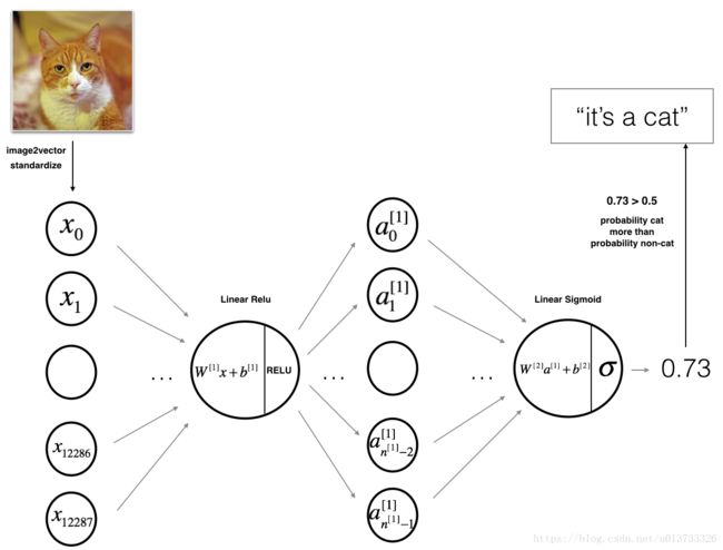
对于一个两层的神经网络结构而言，模型结构是线性->ReLU->线性->sigmod函数。

初始化函数如下：

def initialize_parameters(n_x,n_h,n_y):
    """
    此函数是为了初始化两层网络参数而使用的函数。
    参数：
        n_x - 输入层节点数量
        n_h - 隐藏层节点数量
        n_y - 输出层节点数量
    
    返回：
        parameters - 包含你的参数的python字典：
            W1 - 权重矩阵,维度为（n_h，n_x）
            b1 - 偏向量，维度为（n_h，1）
            W2 - 权重矩阵，维度为（n_y，n_h）
            b2 - 偏向量，维度为（n_y，1）

    """
    W1 = np.random.randn(n_h, n_x) * 0.01
    b1 = np.zeros((n_h, 1))
    W2 = np.random.randn(n_y, n_h) * 0.01
    b2 = np.zeros((n_y, 1))
    
    #使用断言确保我的数据格式是正确的
    assert(W1.shape == (n_h, n_x))
    assert(b1.shape == (n_h, 1))
    assert(W2.shape == (n_y, n_h))
    assert(b2.shape == (n_y, 1))
    
    parameters = {"W1": W1,
                  "b1": b1,
                  "W2": W2,
                  "b2": b2}
    
    return parameters

初始化完成我们来测试一下：

print("==============测试initialize_parameters==============")
parameters = initialize_parameters(3,2,1)
print("W1 = " + str(parameters["W1"]))
print("b1 = " + str(parameters["b1"]))
print("W2 = " + str(parameters["W2"]))
print("b2 = " + str(parameters["b2"]))

测试结果：

==============测试initialize_parameters==============
W1 = [[ 0.01624345 -0.00611756 -0.00528172]
 [-0.01072969  0.00865408 -0.02301539]]
b1 = [[ 0.]
 [ 0.]]
W2 = [[ 0.01744812 -0.00761207]]
b2 = [[ 0.]]

两层的神经网络测试已经完毕了，那么对于一个L层的神经网络而言呢？初始化会是什么样的？

假设X（输入数据）的维度为（12288,209）：


       
     W的维度  
     b的维度   
     激活值的计算
     激活值的维度 



     第 1 层  
     $(n^{[1]},12288)$  
     $(n^{[1]},1)$  
     $Z^{[1]} = W^{[1]}  X + b^{[1]} $  
    
     $(n^{[1]},209)$  



     第 2 层  
     $(n^{[2]}, n^{[1]})$   
     $(n^{[2]},1)$  
    $Z^{[2]} = W^{[2]} A^{[1]} + b^{[2]}$  
     $(n^{[2]}, 209)$  


   
     $\vdots$  
     $\vdots$   
     $\vdots$   
     $\vdots$ 
     $\vdots$

第 L-1 层 $(n^{[L-1]}, n^{[L-2]})$ $(n^{[L-1]}, 1)$ $Z^{[L-1]} = W^{[L-1]} A^{[L-2]} + b^{[L-1]}$ $(n^{[L-1]}, 209)$ 第 L 层 $(n^{[L]}, n^{[L-1]})$ $(n^{[L]}, 1)$ $Z^{[L]} = W^{[L]} A^{[L-1]} + b^{[L]}$ $(n^{[L]}, 209)$

当然，矩阵的计算方法还是要说一下的：
$\begin{bmatrix} j & k & l\\ m & n & o \\ p & q & r \end{bmatrix}\;\;\; X = \begin{bmatrix} a & b & c\\ d & e & f \\ g & h & i \end{bmatrix} \;\;\; b =\begin{bmatrix} s \\ t \\ u \end{bmatrix}\tag{1}$

如果要计算 $W X + b$ 的话，计算方法是这样的：

$\begin{bmatrix} (ja + kd + lg) + s & (jb + ke + lh) + s & (jc + kf + li)+ s\\ (ma + nd + og) + t & (mb + ne + oh) + t & (mc + nf + oi) + t\\ (pa + qd + rg) + u & (pb + qe + rh) + u & (pc + qf + ri)+ u \end{bmatrix}\tag{2}$

在实际中，也不需要你去做这么复杂的运算，我们来看一下它是怎样计算的吧：

def initialize_parameters_deep(layers_dims):
    """
    此函数是为了初始化多层网络参数而使用的函数。
    参数：
        layers_dims - 包含我们网络中每个图层的节点数量的列表
    
    返回：
        parameters - 包含参数“W1”，“b1”，...，“WL”，“bL”的字典：
                     W1 - 权重矩阵，维度为（layers_dims [1]，layers_dims [1-1]）
                     bl - 偏向量，维度为（layers_dims [1]，1）
    """
    np.random.seed(3)
    parameters = {}
    L = len(layers_dims)
    
    for l in range(1,L):
	    parameters["W" + str(l)] = np.random.randn(layers_dims[l], layers_dims[l - 1]) / np.sqrt(layers_dims[l - 1])
        parameters["b" + str(l)] = np.zeros((layers_dims[l], 1))
        
        #确保我要的数据的格式是正确的
        assert(parameters["W" + str(l)].shape == (layers_dims[l], layers_dims[l-1]))
        assert(parameters["b" + str(l)].shape == (layers_dims[l], 1))
        
    return parameters

测试一下：

#测试initialize_parameters_deep
print("==============测试initialize_parameters_deep==============")
layers_dims = [5,4,3]
parameters = initialize_parameters_deep(layers_dims)
print("W1 = " + str(parameters["W1"]))
print("b1 = " + str(parameters["b1"]))
print("W2 = " + str(parameters["W2"]))
print("b2 = " + str(parameters["b2"]))

测试结果：

==============测试initialize_parameters_deep==============
W1 = [[ 0.01788628  0.0043651   0.00096497 -0.01863493 -0.00277388]
 [-0.00354759 -0.00082741 -0.00627001 -0.00043818 -0.00477218]
 [-0.01313865  0.00884622  0.00881318  0.01709573  0.00050034]
 [-0.00404677 -0.0054536  -0.01546477  0.00982367 -0.01101068]]
b1 = [[ 0.]
 [ 0.]
 [ 0.]
 [ 0.]]
W2 = [[-0.01185047 -0.0020565   0.01486148  0.00236716]
 [-0.01023785 -0.00712993  0.00625245 -0.00160513]
 [-0.00768836 -0.00230031  0.00745056  0.01976111]]
b2 = [[ 0.]
 [ 0.]
 [ 0.]]

我们分别构建了两层和多层神经网络的初始化参数的函数，现在我们开始构建前向传播函数。

前向传播函数

前向传播有以下三个步骤

LINEAR
LINEAR - >ACTIVATION，其中激活函数将会使用ReLU或Sigmoid。
[LINEAR - > RELU] ×（L-1） - > LINEAR - > SIGMOID（整个模型）

线性正向传播模块（向量化所有示例）使用公式(3)进行计算：
$Z^{[l]} = W^{[l]}A^{[l-1]} +b^{[l]}\tag{3}$

线性部分【LINEAR】

前向传播中，线性部分计算如下：

def linear_forward(A,W,b):
    """
    实现前向传播的线性部分。

    参数：
        A - 来自上一层（或输入数据）的激活，维度为(上一层的节点数量，示例的数量）
        W - 权重矩阵，numpy数组，维度为（当前图层的节点数量，前一图层的节点数量）
        b - 偏向量，numpy向量，维度为（当前图层节点数量，1）

    返回：
         Z - 激活功能的输入，也称为预激活参数
         cache - 一个包含“A”，“W”和“b”的字典，存储这些变量以有效地计算后向传递
    """
    Z = np.dot(W,A) + b
    assert(Z.shape == (W.shape[0],A.shape[1]))
    cache = (A,W,b)
     
    return Z,cache

测试一下线性部分：

#测试linear_forward
print("==============测试linear_forward==============")
A,W,b = testCases.linear_forward_test_case()
Z,linear_cache = linear_forward(A,W,b)
print("Z = " + str(Z))

测试结果：

==============测试linear_forward==============
Z = [[ 3.26295337 -1.23429987]]

我们前向传播的单层计算完成了一半啦！我们来开始构建后半部分，如果你不知道我在说啥，请往上翻到【开始之前】仔细看看吧~

线性激活部分【LINEAR - >ACTIVATION】

为了更方便，我们将把两个功能（线性和激活）分组为一个功能（LINEAR-> ACTIVATION）。因此，我们将实现一个执行LINEAR前进步骤，然后执行ACTIVATION前进步骤的功能。我们来看看这激活函数的数学实现吧~

Sigmoid: $\sigma(Z) = \sigma(W A + b) = \frac{1}{ 1 + e^{-(W A + b)}}$
ReLU: $A = R E L U (Z) = m a x (0, Z)$

我们为了实现LINEAR->ACTIVATION这个步骤，使用的公式是： $A^{[l]} = g(Z^{[l]}) = g(W^{[l]}A^{[l-1]} +b^{[l]})$ ，其中，函数g会是sigmoid() 或者是 relu()，当然，sigmoid()只在输出层使用,现在我们正式构建前向线性激活部分。

def linear_activation_forward(A_prev,W,b,activation):
    """
    实现LINEAR-> ACTIVATION 这一层的前向传播

    参数：
        A_prev - 来自上一层（或输入层）的激活，维度为(上一层的节点数量，示例数）
        W - 权重矩阵，numpy数组，维度为（当前层的节点数量，前一层的大小）
        b - 偏向量，numpy阵列，维度为（当前层的节点数量，1）
        activation - 选择在此层中使用的激活函数名，字符串类型，【"sigmoid" | "relu"】

    返回：
        A - 激活函数的输出，也称为激活后的值
        cache - 一个包含“linear_cache”和“activation_cache”的字典，我们需要存储它以有效地计算后向传递
    """
    
    if activation == "sigmoid":
        Z, linear_cache = linear_forward(A_prev, W, b)
        A, activation_cache = sigmoid(Z)
    elif activation == "relu":
        Z, linear_cache = linear_forward(A_prev, W, b)
        A, activation_cache = relu(Z)
    
    assert(A.shape == (W.shape[0],A_prev.shape[1]))
    cache = (linear_cache,activation_cache)
    
    return A,cache

测试一下：

#测试linear_activation_forward
print("==============测试linear_activation_forward==============")
A_prev, W,b = testCases.linear_activation_forward_test_case()

A, linear_activation_cache = linear_activation_forward(A_prev, W, b, activation = "sigmoid")
print("sigmoid，A = " + str(A))

A, linear_activation_cache = linear_activation_forward(A_prev, W, b, activation = "relu")
print("ReLU，A = " + str(A))

测试结果：

==============测试linear_activation_forward==============
sigmoid，A = [[ 0.96890023  0.11013289]]
ReLU，A = [[ 3.43896131  0.        ]]

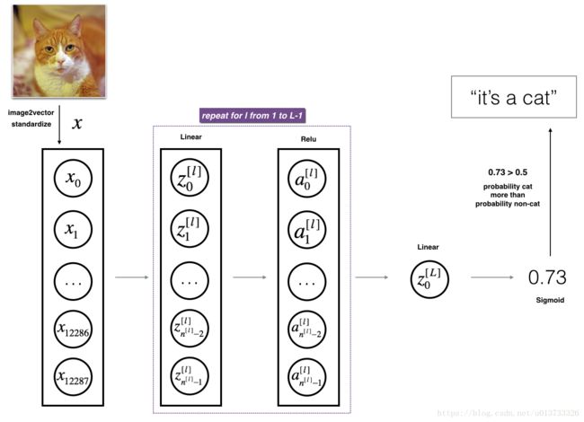
我们把两层模型需要的前向传播函数做完了，那多层网络模型的前向传播是怎样的呢？我们调用上面的那两个函数来实现它，为了在实现L层神经网络时更加方便，我们需要一个函数来复制前一个函数（带有RELU的linear_activation_forward）L-1次，然后用一个带有SIGMOID的linear_activation_forward跟踪它，我们来看一下它的结构是怎样的：

**Figure 2** : *[LINEAR -> RELU] $\times$ (L-1) -> LINEAR -> SIGMOID* model

在下面的代码中，AL表示 $A^{[L]} = \sigma(Z^{[L]}) = \sigma(W^{[L]} A^{[L-1]} + b^{[L]})$ . (也可称作 Yhat,数学表示为 $\hat{Y}$ .)

多层模型的前向传播计算模型代码如下：

def L_model_forward(X,parameters):
    """
    实现[LINEAR-> RELU] *（L-1） - > LINEAR-> SIGMOID计算前向传播，也就是多层网络的前向传播，为后面每一层都执行LINEAR和ACTIVATION
    
    参数：
        X - 数据，numpy数组，维度为（输入节点数量，示例数）
        parameters - initialize_parameters_deep（）的输出
    
    返回：
        AL - 最后的激活值
        caches - 包含以下内容的缓存列表：
                 linear_relu_forward（）的每个cache（有L-1个，索引为从0到L-2）
                 linear_sigmoid_forward（）的cache（只有一个，索引为L-1）
    """
    caches = []
    A = X
    L = len(parameters) // 2
    for l in range(1,L):
        A_prev = A 
        A, cache = linear_activation_forward(A_prev, parameters['W' + str(l)], parameters['b' + str(l)], "relu")
        caches.append(cache)
    
    AL, cache = linear_activation_forward(A, parameters['W' + str(L)], parameters['b' + str(L)], "sigmoid")
    caches.append(cache)
    
    assert(AL.shape == (1,X.shape[1]))
    
    return AL,caches

测试一下：

#测试L_model_forward
print("==============测试L_model_forward==============")
X,parameters = testCases.L_model_forward_test_case()
AL,caches = L_model_forward(X,parameters)
print("AL = " + str(AL))
print("caches 的长度为 = " + str(len(caches)))

测试结果：

==============测试L_model_forward==============
AL = [[ 0.17007265  0.2524272 ]]
caches 的长度为 = 2

计算成本

我们已经把这两个模型的前向传播部分完成了，我们需要计算成本（误差），以确定它到底有没有在学习，成本的计算公式如下：
$-\frac{1}{m} \sum\limits_{i = 1}^{m} (y^{(i)}\log\left(a^{[L] (i)}\right) + (1-y^{(i)})\log\left(1- a^{[L](i)}\right)) \tag{4}$

def compute_cost(AL,Y):
    """
    实施等式（4）定义的成本函数。

    参数：
        AL - 与标签预测相对应的概率向量，维度为（1，示例数量）
        Y - 标签向量（例如：如果不是猫，则为0，如果是猫则为1），维度为（1，数量）

    返回：
        cost - 交叉熵成本
    """
    m = Y.shape[1]
    cost = -np.sum(np.multiply(np.log(AL),Y) + np.multiply(np.log(1 - AL), 1 - Y)) / m
        
    cost = np.squeeze(cost)
    assert(cost.shape == ())

    return cost

测试一下：

#测试compute_cost
print("==============测试compute_cost==============")
Y,AL = testCases.compute_cost_test_case()
print("cost = " + str(compute_cost(AL, Y)))

测试结果：

==============测试compute_cost==============
cost = 0.414931599615

我们已经把误差值计算出来了，现在开始进行反向传播

反向传播

反向传播用于计算相对于参数的损失函数的梯度，我们来看看向前和向后传播的流程图：

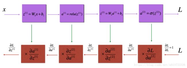
流程图有了，我们再来看一看对于线性的部分的公式：

我们需要使用 $dZ^{[l]}$ 来计算三个输出 $dW^{[l]}, db^{[l]}, dA^{[l]})$ ，下面三个公式是我们要用到的：
$dW^{[l]} = \frac{\partial \mathcal{L} }{\partial W^{[l]}} = \frac{1}{m} dZ^{[l]} A^{[l-1] T} \tag{5}$
$db^{[l]} = \frac{\partial \mathcal{L} }{\partial b^{[l]}} = \frac{1}{m} \sum_{i = 1}^{m} dZ^{[l](i)}\tag{6}$
$dA^{[l-1]} = \frac{\partial \mathcal{L} }{\partial A^{[l-1]}} = W^{[l] T} dZ^{[l]} \tag{7}$

与前向传播类似，我们有需要使用三个步骤来构建反向传播：

LINEAR 后向计算
LINEAR -> ACTIVATION 后向计算，其中ACTIVATION 计算Relu或者Sigmoid 的结果
[LINEAR -> RELU] $\times$ (L-1) -> LINEAR -> SIGMOID 后向计算 (整个模型)

线性部分【LINEAR backward】

我们来实现后向传播线性部分：

def linear_backward(dZ,cache):
    """
    为单层实现反向传播的线性部分（第L层）

    参数：
         dZ - 相对于（当前第l层的）线性输出的成本梯度
         cache - 来自当前层前向传播的值的元组（A_prev，W，b）

    返回：
         dA_prev - 相对于激活（前一层l-1）的成本梯度，与A_prev维度相同
         dW - 相对于W（当前层l）的成本梯度，与W的维度相同
         db - 相对于b（当前层l）的成本梯度，与b维度相同
    """
    A_prev, W, b = cache
    m = A_prev.shape[1]
    dW = np.dot(dZ, A_prev.T) / m
    db = np.sum(dZ, axis=1, keepdims=True) / m
    dA_prev = np.dot(W.T, dZ)
    
    assert (dA_prev.shape == A_prev.shape)
    assert (dW.shape == W.shape)
    assert (db.shape == b.shape)
    
    return dA_prev, dW, db

测试一下：

#测试linear_backward
print("==============测试linear_backward==============")
dZ, linear_cache = testCases.linear_backward_test_case()

dA_prev, dW, db = linear_backward(dZ, linear_cache)
print ("dA_prev = "+ str(dA_prev))
print ("dW = " + str(dW))
print ("db = " + str(db))

测试结果：

==============测试linear_backward==============
dA_prev = [[ 0.51822968 -0.19517421]
 [-0.40506361  0.15255393]
 [ 2.37496825 -0.89445391]]
dW = [[-0.10076895  1.40685096  1.64992505]]
db = [[ 0.50629448]]

线性激活部分【LINEAR -> ACTIVATION backward】

为了帮助你实现linear_activation_backward，我们提供了两个后向函数：

sigmoid_backward:实现了sigmoid（）函数的反向传播，你可以这样调用它：

dZ = sigmoid_backward(dA, activation_cache)

relu_backward: 实现了relu（）函数的反向传播，你可以这样调用它：

dZ = relu_backward(dA, activation_cache)

如果 $g (.)$ 是激活函数, 那么sigmoid_backward 和 relu_backward 这样计算：
$dZ^{[l]} = dA^{[l]} * g'(Z^{[l]}) \tag{8}$ .

我们先在正式开始实现后向线性激活：

def linear_activation_backward(dA,cache,activation="relu"):
    """
    实现LINEAR-> ACTIVATION层的后向传播。
    
    参数：
         dA - 当前层l的激活后的梯度值
         cache - 我们存储的用于有效计算反向传播的值的元组（值为linear_cache，activation_cache）
         activation - 要在此层中使用的激活函数名，字符串类型，【"sigmoid" | "relu"】
    返回：
         dA_prev - 相对于激活（前一层l-1）的成本梯度值，与A_prev维度相同
         dW - 相对于W（当前层l）的成本梯度值，与W的维度相同
         db - 相对于b（当前层l）的成本梯度值，与b的维度相同
    """
    linear_cache, activation_cache = cache
    if activation == "relu":
        dZ = relu_backward(dA, activation_cache)
        dA_prev, dW, db = linear_backward(dZ, linear_cache)
    elif activation == "sigmoid":
        dZ = sigmoid_backward(dA, activation_cache)
        dA_prev, dW, db = linear_backward(dZ, linear_cache)
    
    return dA_prev,dW,db

测试一下：

#测试linear_activation_backward
print("==============测试linear_activation_backward==============")
AL, linear_activation_cache = testCases.linear_activation_backward_test_case()
 
dA_prev, dW, db = linear_activation_backward(AL, linear_activation_cache, activation = "sigmoid")
print ("sigmoid:")
print ("dA_prev = "+ str(dA_prev))
print ("dW = " + str(dW))
print ("db = " + str(db) + "\n")
 
dA_prev, dW, db = linear_activation_backward(AL, linear_activation_cache, activation = "relu")
print ("relu:")
print ("dA_prev = "+ str(dA_prev))
print ("dW = " + str(dW))
print ("db = " + str(db))

测试结果：

==============测试linear_activation_backward==============
sigmoid:
dA_prev = [[ 0.11017994  0.01105339]
 [ 0.09466817  0.00949723]
 [-0.05743092 -0.00576154]]
dW = [[ 0.10266786  0.09778551 -0.01968084]]
db = [[-0.05729622]]

relu:
dA_prev = [[ 0.44090989 -0.        ]
 [ 0.37883606 -0.        ]
 [-0.2298228   0.        ]]
dW = [[ 0.44513824  0.37371418 -0.10478989]]
db = [[-0.20837892]]

我们已经把两层模型的后向计算完成了，对于多层模型我们也需要这两个函数来完成，我们来看一下流程图：

在之前的前向计算中，我们存储了一些包含包含（X，W，b和z）的cache，在犯下那个船舶中，我们将会使用它们来计算梯度值，所以，在L层模型中，我们需要从L层遍历所有的隐藏层，在每一步中，我们需要使用那一层的cache值来进行反向传播。
上面我们提到了 $A^{[L]}$ ，它属于输出层， $A^{[L]} = \sigma(Z^{[L]})$ ，所以我们需要计算dAL，我们可以使用下面的代码来计算它：

dAL = - (np.divide(Y, AL) - np.divide(1 - Y, 1 - AL))

计算完了以后，我们可以使用此激活后的梯度dAL继续向后计算，我们这就开始构建多层模型向后传播函数：

def L_model_backward(AL,Y,caches):
    """
    对[LINEAR-> RELU] *（L-1） - > LINEAR - > SIGMOID组执行反向传播，就是多层网络的向后传播
    
    参数：
     AL - 概率向量，正向传播的输出（L_model_forward（））
     Y - 标签向量（例如：如果不是猫，则为0，如果是猫则为1），维度为（1，数量）
     caches - 包含以下内容的cache列表：
                 linear_activation_forward（"relu"）的cache，不包含输出层
                 linear_activation_forward（"sigmoid"）的cache
    
    返回：
     grads - 具有梯度值的字典
              grads [“dA”+ str（l）] = ...
              grads [“dW”+ str（l）] = ...
              grads [“db”+ str（l）] = ...
    """
    grads = {}
    L = len(caches)
    m = AL.shape[1]
    Y = Y.reshape(AL.shape)
    dAL = - (np.divide(Y, AL) - np.divide(1 - Y, 1 - AL))
    
    current_cache = caches[L-1]
    grads["dA" + str(L)], grads["dW" + str(L)], grads["db" + str(L)] = linear_activation_backward(dAL, current_cache, "sigmoid")
    
    for l in reversed(range(L-1)):
        current_cache = caches[l]
        dA_prev_temp, dW_temp, db_temp = linear_activation_backward(grads["dA" + str(l + 2)], current_cache, "relu")
        grads["dA" + str(l + 1)] = dA_prev_temp
        grads["dW" + str(l + 1)] = dW_temp
        grads["db" + str(l + 1)] = db_temp
    
    return grads

测试一下：

#测试L_model_backward
print("==============测试L_model_backward==============")
AL, Y_assess, caches = testCases.L_model_backward_test_case()
grads = L_model_backward(AL, Y_assess, caches)
print ("dW1 = "+ str(grads["dW1"]))
print ("db1 = "+ str(grads["db1"]))
print ("dA1 = "+ str(grads["dA1"]))

测试结果：

==============测试L_model_backward==============
dW1 = [[ 0.41010002  0.07807203  0.13798444  0.10502167]
 [ 0.          0.          0.          0.        ]
 [ 0.05283652  0.01005865  0.01777766  0.0135308 ]]
db1 = [[-0.22007063]
 [ 0.        ]
 [-0.02835349]]
dA1 = [[ 0.          0.52257901]
 [ 0.         -0.3269206 ]
 [ 0.         -0.32070404]
 [ 0.         -0.74079187]]

更新参数

我们把向前向后传播都完成了，现在我们就开始更新参数，当然，我们来看看更新参数的公式吧~

$W^{[l]} = W^{[l]} - \alpha \text{ } dW^{[l]} \tag{9}$
$b^{[l]} = b^{[l]} - \alpha \text{ } db^{[l]} \tag{10}$

其中 $\alpha$ 是学习率。

def update_parameters(parameters, grads, learning_rate):
    """
    使用梯度下降更新参数
    
    参数：
     parameters - 包含你的参数的字典
     grads - 包含梯度值的字典，是L_model_backward的输出
    
    返回：
     parameters - 包含更新参数的字典
                   参数[“W”+ str（l）] = ...
                   参数[“b”+ str（l）] = ...
    """
    L = len(parameters) // 2 #整除
    for l in range(L):
        parameters["W" + str(l + 1)] = parameters["W" + str(l + 1)] - learning_rate * grads["dW" + str(l + 1)]
        parameters["b" + str(l + 1)] = parameters["b" + str(l + 1)] - learning_rate * grads["db" + str(l + 1)]
        
    return parameters

测试一下：

#测试update_parameters
print("==============测试update_parameters==============")
parameters, grads = testCases.update_parameters_test_case()
parameters = update_parameters(parameters, grads, 0.1)
 
print ("W1 = "+ str(parameters["W1"]))
print ("b1 = "+ str(parameters["b1"]))
print ("W2 = "+ str(parameters["W2"]))
print ("b2 = "+ str(parameters["b2"]))

测试结果：

==============测试update_parameters==============
W1 = [[-0.59562069 -0.09991781 -2.14584584  1.82662008]
 [-1.76569676 -0.80627147  0.51115557 -1.18258802]
 [-1.0535704  -0.86128581  0.68284052  2.20374577]]
b1 = [[-0.04659241]
 [-1.28888275]
 [ 0.53405496]]
W2 = [[-0.55569196  0.0354055   1.32964895]]
b2 = [[-0.84610769]]

至此为止，我们已经实现该神经网络中所有需要的函数。接下来，我们将这些方法组合在一起，构成一个神经网络类，可以方便的使用。

搭建两层神经网络

一个两层的神经网络模型图如下：

该模型可以概括为： **INPUT -> LINEAR -> RELU -> LINEAR -> SIGMOID -> OUTPUT**

我们正式开始构建两层的神经网络:

def two_layer_model(X,Y,layers_dims,learning_rate=0.0075,num_iterations=3000,print_cost=False,isPlot=True):
    """
    实现一个两层的神经网络，【LINEAR->RELU】 -> 【LINEAR->SIGMOID】
    参数：
        X - 输入的数据，维度为(n_x，例子数)
        Y - 标签，向量，0为非猫，1为猫，维度为(1,数量)
        layers_dims - 层数的向量，维度为(n_y,n_h,n_y)
        learning_rate - 学习率
        num_iterations - 迭代的次数
        print_cost - 是否打印成本值，每100次打印一次
        isPlot - 是否绘制出误差值的图谱
    返回:
        parameters - 一个包含W1，b1，W2，b2的字典变量
    """
    np.random.seed(1)
    grads = {}
    costs = []
    (n_x,n_h,n_y) = layers_dims
    
    """
    初始化参数
    """
    parameters = initialize_parameters(n_x, n_h, n_y)
    
    W1 = parameters["W1"]
    b1 = parameters["b1"]
    W2 = parameters["W2"]
    b2 = parameters["b2"]
    
    """
    开始进行迭代
    """
    for i in range(0,num_iterations):
        #前向传播
        A1, cache1 = linear_activation_forward(X, W1, b1, "relu")
        A2, cache2 = linear_activation_forward(A1, W2, b2, "sigmoid")
        
        #计算成本
        cost = compute_cost(A2,Y)
        
        #后向传播
        ##初始化后向传播
        dA2 = - (np.divide(Y, A2) - np.divide(1 - Y, 1 - A2))
        
        ##向后传播，输入：“dA2，cache2，cache1”。 输出：“dA1，dW2，db2;还有dA0（未使用），dW1，db1”。
        dA1, dW2, db2 = linear_activation_backward(dA2, cache2, "sigmoid")
        dA0, dW1, db1 = linear_activation_backward(dA1, cache1, "relu")
        
        ##向后传播完成后的数据保存到grads
        grads["dW1"] = dW1
        grads["db1"] = db1
        grads["dW2"] = dW2
        grads["db2"] = db2
        
        #更新参数
        parameters = update_parameters(parameters,grads,learning_rate)
        W1 = parameters["W1"]
        b1 = parameters["b1"]
        W2 = parameters["W2"]
        b2 = parameters["b2"]
        
        #打印成本值，如果print_cost=False则忽略
        if i % 100 == 0:
            #记录成本
            costs.append(cost)
            #是否打印成本值
            if print_cost:
                print("第", i ,"次迭代，成本值为：" ,np.squeeze(cost))
    #迭代完成，根据条件绘制图
    if isPlot:
        plt.plot(np.squeeze(costs))
        plt.ylabel('cost')
        plt.xlabel('iterations (per tens)')
        plt.title("Learning rate =" + str(learning_rate))
        plt.show()
    
    #返回parameters
    return parameters

我们现在开始加载数据集,图像数据集的处理可以参照：【中文】【吴恩达课后编程作业】Course 1 - 神经网络和深度学习 - 第二周作业，就连数据集也是一样的。

train_set_x_orig , train_set_y , test_set_x_orig , test_set_y , classes = lr_utils.load_dataset()

train_x_flatten = train_set_x_orig.reshape(train_set_x_orig.shape[0], -1).T 
test_x_flatten = test_set_x_orig.reshape(test_set_x_orig.shape[0], -1).T

train_x = train_x_flatten / 255
train_y = train_set_y
test_x = test_x_flatten / 255
test_y = test_set_y

数据集加载完成，开始正式训练：

n_x = 12288
n_h = 7
n_y = 1
layers_dims = (n_x,n_h,n_y)

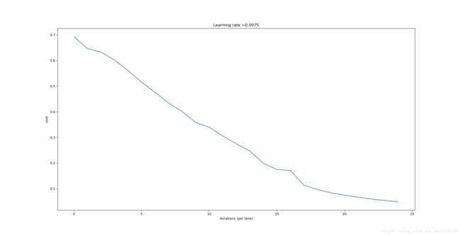
parameters = two_layer_model(train_x, train_set_y, layers_dims = (n_x, n_h, n_y), num_iterations = 2500, print_cost=True,isPlot=True)

训练结果：

第 0 次迭代，成本值为： 0.69304973566
第 100 次迭代，成本值为： 0.646432095343
第 200 次迭代，成本值为： 0.632514064791
第 300 次迭代，成本值为： 0.601502492035
第 400 次迭代，成本值为： 0.560196631161
第 500 次迭代，成本值为： 0.515830477276
第 600 次迭代，成本值为： 0.475490131394
第 700 次迭代，成本值为： 0.433916315123
第 800 次迭代，成本值为： 0.40079775362
第 900 次迭代，成本值为： 0.358070501132
第 1000 次迭代，成本值为： 0.339428153837
第 1100 次迭代，成本值为： 0.30527536362
第 1200 次迭代，成本值为： 0.274913772821
第 1300 次迭代，成本值为： 0.246817682106
第 1400 次迭代，成本值为： 0.198507350375
第 1500 次迭代，成本值为： 0.174483181126
第 1600 次迭代，成本值为： 0.170807629781
第 1700 次迭代，成本值为： 0.113065245622
第 1800 次迭代，成本值为： 0.0962942684594
第 1900 次迭代，成本值为： 0.0834261795973
第 2000 次迭代，成本值为： 0.0743907870432
第 2100 次迭代，成本值为： 0.0663074813227
第 2200 次迭代，成本值为： 0.0591932950104
第 2300 次迭代，成本值为： 0.0533614034856
第 2400 次迭代，成本值为： 0.0485547856288

迭代完成之后我们就可以进行预测了，预测函数如下：

def predict(X, y, parameters):
    """
    该函数用于预测L层神经网络的结果，当然也包含两层
    
    参数：
     X - 测试集
     y - 标签
     parameters - 训练模型的参数
    
    返回：
     p - 给定数据集X的预测
    """
    
    m = X.shape[1]
    n = len(parameters) // 2 # 神经网络的层数
    p = np.zeros((1,m))
    
    #根据参数前向传播
    probas, caches = L_model_forward(X, parameters)
    
    for i in range(0, probas.shape[1]):
        if probas[0,i] > 0.5:
            p[0,i] = 1
        else:
            p[0,i] = 0
    
    print("准确度为: "  + str(float(np.sum((p == y))/m)))
        
    return p

预测函数构建好了我们就开始预测，查看训练集和测试集的准确性：

predictions_train = predict(train_x, train_y, parameters) #训练集
predictions_test = predict(test_x, test_y, parameters) #测试集

预测结果：

准确度为: 1.0
准确度为: 0.72

这样看来，我的测试集的准确度要比上一次（【中文】【吴恩达课后编程作业】Course 1 - 神经网络和深度学习 - 第二周作业）高一些，上次的是70%，这次是72%，那如果我使用更多层的圣经网络呢？

搭建多层神经网络

我们首先来看看多层的网络的结构吧~

def L_layer_model(X, Y, layers_dims, learning_rate=0.0075, num_iterations=3000, print_cost=False,isPlot=True):
    """
    实现一个L层神经网络：[LINEAR-> RELU] *（L-1） - > LINEAR-> SIGMOID。
    
    参数：
	    X - 输入的数据，维度为(n_x，例子数)
        Y - 标签，向量，0为非猫，1为猫，维度为(1,数量)
        layers_dims - 层数的向量，维度为(n_y,n_h,···,n_h,n_y)
        learning_rate - 学习率
        num_iterations - 迭代的次数
        print_cost - 是否打印成本值，每100次打印一次
        isPlot - 是否绘制出误差值的图谱
    
    返回：
     parameters - 模型学习的参数。 然后他们可以用来预测。
    """
    np.random.seed(1)
    costs = []
    
    parameters = initialize_parameters_deep(layers_dims)
    
    for i in range(0,num_iterations):
        AL , caches = L_model_forward(X,parameters)
        
        cost = compute_cost(AL,Y)
        
        grads = L_model_backward(AL,Y,caches)
        
        parameters = update_parameters(parameters,grads,learning_rate)
        
        #打印成本值，如果print_cost=False则忽略
        if i % 100 == 0:
            #记录成本
            costs.append(cost)
            #是否打印成本值
            if print_cost:
                print("第", i ,"次迭代，成本值为：" ,np.squeeze(cost))
    #迭代完成，根据条件绘制图
    if isPlot:
        plt.plot(np.squeeze(costs))
        plt.ylabel('cost')
        plt.xlabel('iterations (per tens)')
        plt.title("Learning rate =" + str(learning_rate))
        plt.show()
    return parameters

train_set_x_orig , train_set_y , test_set_x_orig , test_set_y , classes = lr_utils.load_dataset()

train_x_flatten = train_set_x_orig.reshape(train_set_x_orig.shape[0], -1).T 
test_x_flatten = test_set_x_orig.reshape(test_set_x_orig.shape[0], -1).T

train_x = train_x_flatten / 255
train_y = train_set_y
test_x = test_x_flatten / 255
test_y = test_set_y

数据集加载完成，开始正式训练：

layers_dims = [12288, 20, 7, 5, 1] #  5-layer model
parameters = L_layer_model(train_x, train_y, layers_dims, num_iterations = 2500, print_cost = True,isPlot=True)

训练结果：

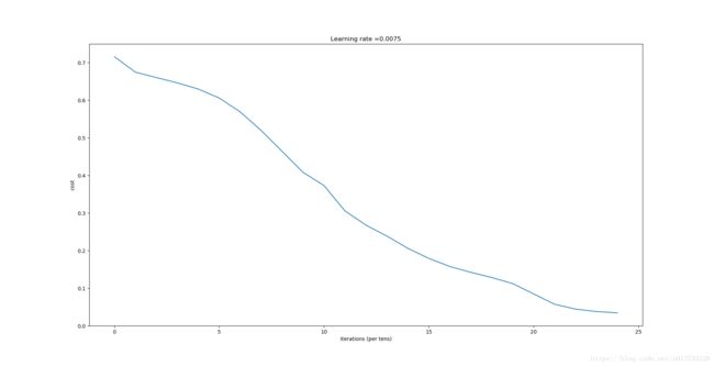
第 0 次迭代，成本值为： 0.715731513414
第 100 次迭代，成本值为： 0.674737759347
第 200 次迭代，成本值为： 0.660336543362
第 300 次迭代，成本值为： 0.646288780215
第 400 次迭代，成本值为： 0.629813121693
第 500 次迭代，成本值为： 0.606005622927
第 600 次迭代，成本值为： 0.569004126398
第 700 次迭代，成本值为： 0.519796535044
第 800 次迭代，成本值为： 0.464157167863
第 900 次迭代，成本值为： 0.408420300483
第 1000 次迭代，成本值为： 0.373154992161
第 1100 次迭代，成本值为： 0.30572374573
第 1200 次迭代，成本值为： 0.268101528477
第 1300 次迭代，成本值为： 0.238724748277
第 1400 次迭代，成本值为： 0.206322632579
第 1500 次迭代，成本值为： 0.179438869275
第 1600 次迭代，成本值为： 0.157987358188
第 1700 次迭代，成本值为： 0.142404130123
第 1800 次迭代，成本值为： 0.128651659979
第 1900 次迭代，成本值为： 0.112443149982
第 2000 次迭代，成本值为： 0.0850563103497
第 2100 次迭代，成本值为： 0.0575839119861
第 2200 次迭代，成本值为： 0.044567534547
第 2300 次迭代，成本值为： 0.038082751666
第 2400 次迭代，成本值为： 0.0344107490184

训练完成，我们看一下预测：

pred_train = predict(train_x, train_y, parameters) #训练集
pred_test = predict(test_x, test_y, parameters) #测试集

预测结果：

准确度为: 0.9952153110047847
准确度为: 0.78

就准确度而言，从70%到72%再到78%，可以看到的是准确度在一点点增加，当然，你也可以手动的去调整layers_dims，准确度可能又会提高一些。

分析

我们可以看一看有哪些东西在L层模型中被错误地标记了，导致准确率没有提高。

def print_mislabeled_images(classes, X, y, p):
    """
	绘制预测和实际不同的图像。
	    X - 数据集
	    y - 实际的标签
	    p - 预测
    """
    a = p + y
    mislabeled_indices = np.asarray(np.where(a == 1))
    plt.rcParams['figure.figsize'] = (40.0, 40.0) # set default size of plots
    num_images = len(mislabeled_indices[0])
    for i in range(num_images):
        index = mislabeled_indices[1][i]
        
        plt.subplot(2, num_images, i + 1)
        plt.imshow(X[:,index].reshape(64,64,3), interpolation='nearest')
        plt.axis('off')
        plt.title("Prediction: " + classes[int(p[0,index])].decode("utf-8") + " \n Class: " + classes[y[0,index]].decode("utf-8"))


print_mislabeled_images(classes, test_x, test_y, pred_test)

运行结果：

分析一下我们就可以得知原因了：
模型往往表现欠佳的几种类型的图像包括：

猫身体在一个不同的位置
猫出现在相似颜色的背景下
不同的猫的颜色和品种
相机角度
图片的亮度
比例变化（猫的图像非常大或很小）

【选做】

我们使用自己图片试试？
我们把一张图片放在一个特定位置，然后识别它。


## START CODE HERE ##
my_image = "my_image.jpg" # change this to the name of your image file 
my_label_y = [1] # the true class of your image (1 -> cat, 0 -> non-cat)
## END CODE HERE ##

fname = "images/" + my_image
image = np.array(ndimage.imread(fname, flatten=False))
my_image = scipy.misc.imresize(image, size=(num_px,num_px)).reshape((num_px*num_px*3,1))
my_predicted_image = predict(my_image, my_label_y, parameters)

plt.imshow(image)
print ("y = " + str(np.squeeze(my_predicted_image)) + ", your L-layer model predicts a \"" + classes[int(np.squeeze(my_predicted_image)),].decode("utf-8") +  "\" picture.")

运行结果：

准确度: 1.0
y = 1.0, your L-layer model predicts a "cat" picture.

【中文】【吴恩达课后编程作业】Course 1 - 神经网络和深度学习 - 第四周作业(1&2)

【吴恩达课后编程作业】01 - 神经网络和深度学习 - 第四周 - PA1&2 - 一步步搭建多层神经网络以及应用

声明

开始之前

准备软件包

初始化参数

前向传播函数

线性部分【LINEAR】

线性激活部分【LINEAR - >ACTIVATION】

计算成本

反向传播

线性部分【LINEAR backward】

线性激活部分【LINEAR -> ACTIVATION backward】

更新参数

搭建两层神经网络

搭建多层神经网络

分析

【选做】

相关库代码

lr_utils.py

dnn_utils.py

testCase.py

你可能感兴趣的:(吴恩达的课后作业)