和我一起搭建神经网络——利用Logistics回归实现猫的识别

第一步：数据的导入与预处理

为了完成搭建识别猫的这样一个神经网络，我们先看看程序中需要import哪些库：

1. numpy ：是用Python进行科学计算的基本软件包
2. h5py：是与H5文件中存储的数据集进行交互的常用软件包
3. matplotlib：是一个著名的库，用于在Python中绘制图表
4. lr_utils ：在本文的资料包里，一个加载资料包里面的数据的简单功能的库

本程序所需要的资源读者们可以去我的资源里下载：
或者这个网站：https://github.com/Kulbear/deep-learning-coursera/blob/master/Neural Networks and Deep Learning/Logistic Regression with a Neural Network mindset.ipynb
文件名为lr_utils.py和datasets
在编写代码前，请确保您的这些文件和代码文件处于同一工程目录下

import numpy as np
import h5py
import matplotlib.import matplotlib.pyplot as plt
from lr_utils import load_dataset

关于函数load_dataset()的解释，博主参考了下面这篇文章：
https://blog.csdn.net/u013733326/article/details/79639509

def load_dataset():
    train_dataset = h5py.File('datasets/train_catvnoncat.h5', "r")
    train_set_x_orig = np.array(train_dataset["train_set_x"][:]) # your train set features
    train_set_y_orig = np.array(train_dataset["train_set_y"][:]) # your train set labels
    
    test_dataset = h5py.File('datasets/test_catvnoncat.h5', "r")
    test_set_x_orig = np.array(test_dataset["test_set_x"][:]) # your test set features
    test_set_y_orig = np.array(test_dataset["test_set_y"][:]) # your test set labels

    classes = np.array(test_dataset["list_classes"][:]) # the list of classes

    train_set_y_orig = train_set_y_orig.reshape((1, train_set_y_orig.shape[0]))
    test_set_y_orig = test_set_y_orig.reshape((1, test_set_y_orig.shape[0]))
    
    return train_set_x_orig, train_set_y_orig, test_set_x_orig, test_set_y_orig, classes

train_set_x_orig ：保存的是训练集里面的图像数据（本训练集有209张64x64的图像）
train_set_y_orig ：保存的是训练集的图像对应的分类值（【0 | 1】，0表示不是猫，1表示是猫）
test_set_x_orig ：保存的是测试集里面的图像数据（本训练集有50张64x64的图像）
test_set_y_orig ： 保存的是测试集的图像对应的分类值（【0 | 1】，0表示不是猫，1表示是猫)
classes ： 保存的是以bytes类型保存的两个字符串数据，数据为：[b’non-cat’ b’cat’]

我们需要把这些数据载入到我们的程序当中：

train_set_x_orig , train_set_y , test_set_x_orig , test_set_y , classes = load_dataset()

train_set表示训练集
test_set表示测试集

我们想先看看训练集图片（train_set_x_orig）的维数：

print(train_set_x_orig.shape)

输出结果为：(209, 64, 64, 3)
回顾一下吴恩达老师的视频，关于图片的处理是怎么样的？

由于我们载入的图片是RGB三通道的，然后每个通道的图片大小都是64x64，而在视频中我们了解到，每个通道图片的每个像素都是这幅RGB图片的特征，对于特征我们是应该要按行排，对于不同的样本，我们按列排

所以，对于train_set_x_orig，我们把它变为维度为(64 * 64 * 3, 1)会更便于处理

#将训练集的维度降低并转置。
train_set_x_flatten  = train_set_x_orig.reshape(train_set_x_orig.shape[0],-1).T
#将测试集的维度降低并转置。
test_set_x_flatten = test_set_x_orig.reshape(test_set_x_orig.shape[0], -1).T

现在我们再来看看处理之后的train_set_x_flatten和test_set_x_flatten维度是多少：

print(train_set_x_flatten.shape)
print(test_set_x_flatten.shape)

输出：(12288, 209)
         （12288, 50)

机器学习中一个常见的预处理步骤是对数据集进行居中和标准化，对于图片数据集，我们几乎可以将数据集的每一行除以255，因为在RGB中不存在比255大的数据，所以我们可以放心的除以255，让标准化的数据位于[0,1]之间
那么，下面来标准化一下我们的数据：

train_set_x = train_set_x_flatten / 255
test_set_x = test_set_x_flatten / 255

好啦，我们的第一步终于完成啦，其实这一步数据处理也还是挺麻烦的，下面到了有趣的部分：设计神经网络

第二步：设计神经网络以及它们的计算

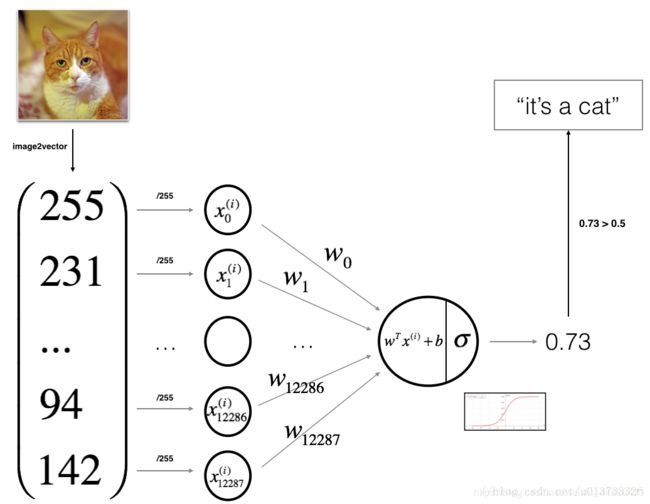
我们这里“输入层”（其实这个说法不太准确，因为在吴恩达老师的视频中曾经讲过，我们习惯把第一个隐藏层当作第一层，但是为了便于理解，我们把输入那块儿就暂且称之为输入层）
我们输入层有12288个神经元（有几个特征就有几个神经元），然后直接传给一个神经元计算预测值，我们在最后采用sigmoid激活函数，因为我们最后的预测值是一种概率形式，分布于[0,1]所以可以使用sigmoid函数

2.1 定义sigmoid函数

def sigmoid(Z):
    A = 1 / (1 + np.exp(-Z))
    return A

2.2 初始化W矩阵和b

def initializer_W_b(dims):
    W = np.zeros(shape = (dims, 1))
    b = 0
    return (W, b)

为什么把W矩阵设置为这个维度呢？我们再回顾一下吴恩达老师的视频课件

红色圈圈圈出来的部分就是W.T矩阵的构建方式：列数代表前一层神经元数量（在本次作业中，前一层就是输入层，神经元数量就是样本的特征数量），行数代表本层神经元的数量（在本次作业中，只有一个神经元)
因此W矩阵的维度就应该是(dims,1)
令b = 0，因为在相加时会出发python的广播机制

2.3 定义前向和反向传播

def propatage(X, Y, W, b):
    m = X.shape[1]    #图片的数量
    A = sigmoid(np.dot(W.T, X) + b)
    cost = (- 1 / m) * np.sum(Y * np.log(A) + (1 - Y) * (np.log(1 - A))) #计算成本，采用交叉熵损失函数

    db = (1 / m) * np.sum(A - Y)
    dW = (1 / m) * np.dot(W, (A - Y).T)
 
    cost = np.squeeze(cost)
    # 我们构造一个字典来存放dW和db:
    grads = {"dW" : dW, "db" : db}
    return (grads, cost)

2.4 定义优化函数，优化权值和偏置

def optimizer(X, Y, W, b, num_iterations , learning_rate, print_cost = False):
    costs = []  #构造一个列表来存放cost
    for i in range(num_iterations):
        grads, cost = propatage(X, Y, W, b)
        dW = grads["dW"]
        db = grads["db"]
        #梯度下降法：
        W = W - learning_rate * dW
        b = b - learning_rate * db
        if i % 100 == 0:
            costs.append(cost)
        if (print_cost) and (i % 100 == 0):
            print("迭代的次数: %i ， 误差值： %f" % (i,cost))
    paras = {"W": W, "b": b}
    grads = {"dW" : dW, "db": db}
    return (paras, grads, costs)

用向量化的方式能大大提高程序的计算速度，去除for循环，但是对于迭代梯度下降的那个for循环暂时还没办法去掉

2.5 定义用于预测的函数prediction

def prediction(W, b, X_test):
    Y_prediction = np.zeros(shape = (1, X_test.shape[1]))
    A = sigmoid(np.dot(W.T, X_test) + b)
    for i in range(A.shape[1]):
        Y_prediction[0,i] = 1 if A[0,i] > 0.5 else 0   #概率大于0.5我们就认为它是猫，设置为1
    return Y_prediction

2.5 设置训练和预测函数

def model(X, Y, X_test, num_iterations, learning_rate):
    W, b = initializer_W_b(X.shape[0])
    paras, grads, costs = optimize(W,b,X,Y,num_iterations , learning_rate, print_cost = True)
    W = paras["W"]  ##从字典中检索W和b
    b = paras["b"]
    Y_prediction = prediction(W, b, X_test)
    return Y_prediction

第三步：调用

Y_prediction = model(train_set_x, train_set_y, test_set_x, 1000, 0.005)
print(Y_prediction)

那么我们来看看自己设计的神经网络的工作效果吧！！！激动人心的时刻！

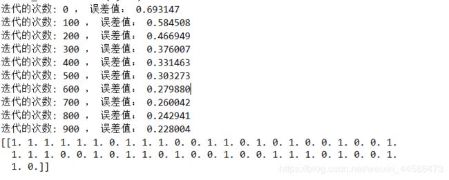
能看到误差值在逐渐减小
下面这个矩阵是我们的神经网络对test图片集的预测，我们来验证一下神经网预测的准确性吧：
它说6张图片不是猫，我们看看哈：

index = 6
plt.imshow(test_set_x_orig[index])

诶呀，真尴尬，预测错误
再看看其他的怎么样：
它说第14张图片不是猫，我们来看看（紧张）：

index = 14
plt.imshow(test_set_x_orig[index])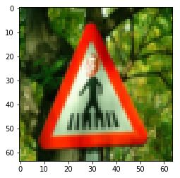

终于对了哈哈
总的来说，这个神经网络预测的准确性一般般，还有很大的提升空间啊

作业中有疑惑的地方：

这个部分是博主目前遇到的一些不解的地方，希望大家能在评论区给出高见，我也会继续查看CSDN博文，如果解决了，我会在第一时间发布解决方案

1. 本程序中使用的学习率是0.005，但是当我把学习率改成0.05或者0.5还是其他什么比1小的数字的时候，会出现这样的情况：

C:/Users/ZZH/.spyder-py3/cat_regonize/NNpractice_catRegonize.py:61: RuntimeWarning: divide by zero encountered in log
cost = (- 1 / m) * np.sum(Y * np.log(A) + (1 - Y) * (np.log(1 - A))) #计算成本
C:/Users/ZZH/.spyder-py3/cat_regonize/NNpractice_catRegonize.py:61: RuntimeWarning: invalid value encountered in multiply
cost = (- 1 / m) * np.sum(Y * np.log(A) + (1 - Y) * (np.log(1 - A))) #计算成本
C:/Users/ZZH/.spyder-py3/cat_regonize/NNpractice_catRegonize.py:46: RuntimeWarning: overflow encountered in exp
a = 1/(1 + np.exp(-z))
迭代的次数: 100 ， 误差值： nan
迭代的次数: 200 ， 误差值： nan
迭代的次数: 300 ， 误差值： nan
迭代的次数: 400 ， 误差值： nan
迭代的次数: 500 ， 误差值： nan
迭代的次数: 600 ， 误差值： nan
迭代的次数: 700 ， 误差值： nan
迭代的次数: 800 ， 误差值： nan
迭代的次数: 900 ， 误差值： nan

2. 把train_set_x_orig，我们把它变为维度为(64 * 64 * 3, 1)时，如果用下面的方法：

#将训练集的维度降低并转置。
train_set_x_flatten  = train_set_x_orig.reshape(12288, 209)
#将测试集的维度降低并转置。
test_set_x_flatten = test_set_x_orig.reshape(12288,50)

会出现这样的情况：
迭代的次数: 100 ， 误差值： 139.462094
迭代的次数: 200 ， 误差值： nan
迭代的次数: 300 ， 误差值： nan
迭代的次数: 400 ， 误差值： 55.380303
迭代的次数: 500 ， 误差值： 87.397194
迭代的次数: 600 ， 误差值： nan
迭代的次数: 700 ， 误差值： nan
迭代的次数: 800 ， 误差值： 63.260267
迭代的次数: 900 ， 误差值： nan
[[0. 0. 0. 0. 0. 0. 0. 0. 0. 0. 0. 0. 0. 0. 0. 0. 0. 0. 0. 0. 0. 0. 0. 0.
0. 0. 0. 0. 0. 0. 0. 0. 0. 0. 0. 0. 0. 0. 0. 0. 0. 0. 0. 0. 0. 0. 0. 0.
0. 0.]]

下面附上源代码：

#-*- coding: utf-8 -*-
import numpy as np
import matplotlib.pyplot as plt
import h5py
from lr_utils import load_dataset

train_set_x_orig , train_set_y , test_set_x_orig , test_set_y , classes = load_dataset()

#将训练集的维度降低并转置。
train_set_x_flatten  = train_set_x_orig.reshape(train_set_x_orig.shape[0],-1).T
#将测试集的维度降低并转置。
test_set_x_flatten = test_set_x_orig.reshape(test_set_x_orig.shape[0],-1).T
train_set_x = train_set_x_flatten / 255
test_set_x = test_set_x_flatten / 255

def sigmoid(z):
    a = 1/(1 + np.exp(-z))
    return a

def initializer_W_b(dims):
    W = np.zeros(shape = (dims,1))   #dims代表样本的特征数
    b = 0
    assert(W.shape == (dims, 1))
    assert(isinstance(b, float) or isinstance(b, int)) #b的类型是float或者是int
    return (W, b)

def protatage(W,b,X,Y):
    m = X.shape[1] #图片的数量
    A = sigmoid(np.dot(W.T,X)+b)
    cost = (- 1 / m) * np.sum(Y * np.log(A) + (1 - Y) * (np.log(1 - A))) #计算成本

    dW = (1/m) * np.dot(X, (A-Y).T)
    db =(1/m) * np.sum(A - Y)
    
    cost = np.squeeze(cost)
    grads = {"dW":dW, "db":db}
    return (grads, cost)

def optimize(W,b,X,Y,num_iterations , learning_rate, print_cost = False):
    costs = []
    for i in range(num_iterations):
        grads,cost = protatage(W,b,X,Y)
        dW = grads["dW"]
        db = grads["db"]
 
        W = W - learning_rate * dW
        b = b - learning_rate * db

        if i % 100 == 0:
            #每隔十次记录一下损失值
            costs.append(cost)  
        if (print_cost) and (i % 100 == 0):
            print("迭代的次数: %i ， 误差值： %f" % (i,cost))

        paras = {"W": W, "b": b}
        grads = {"dW": dW, "db": db}
    return(paras, grads, costs)

def prediction(W, b, X_test):
    Y_prediction = np.zeros(shape = (1,X_test.shape[1]))
    A = sigmoid( np.dot(W.T, X_test)+b)
    for i in range(A.shape[1]):
        Y_prediction[0,i] = 1 if A[0,i] > 0.5 else 0

    return Y_prediction

def model(X, Y, X_test, num_iterations, learning_rate):
    W, b = initializer_W_b(X.shape[0])
    paras, grads, costs = optimize(W,b,X,Y,num_iterations , learning_rate, print_cost = True)
    W = paras["W"]
    b = paras["b"]
    Y_prediction = prediction(W, b, X_test)
    return Y_prediction

Y_prediction = model(train_set_x, train_set_y, test_set_x, 1000, 0.005)
print(Y_prediction)

总的来说，这次的作业让我收获颇丰，虽然也遇到了很多问题和奇奇怪怪的bug，但是亲自实现了构建神经网络的细节，梯度下降的算法等等，之前在Tensorflow上写一些简单的神经网络时，很多时候都直接调用里面的梯度下降函数了，这次终于自己实现了一波，很开心，调试过程也持续了好久，希望在未来神经网络和深度学习的路上能越走越远！