MCMC（Markov Chain Monte Carlo）的理解与实践（Python）

Markov Chain Monte Carlo (MCMC) methods are a class of algorithms for sampling from a probability distribution based on constructing a Markov chain that has the desired distribution as its stationary distribution. The state of the chain after a number of steps is then used as a sample of the desired distribution. The quality of the sample improves as a function of the number of steps.

With MCMC, we draw samples from a (simple) proposal distribution so that each draw depends only on the state of the previous draw (i.e. the samples form a Markov chain, θp=θ+Δθ,Δθ∼N(0,σ) ).

理解MCMC及一系列改进采样算法的关键在于对马尔科夫随机过程的理解。更多详尽的讨论请参见 重温马尔科夫随机过程。

对于给定的概率分布 π(x) ，我们希望能有便捷的方式生成它（ π(x) ）对应的样本。由于马氏链能收敛到平稳分布，于是一个很nice的想法（by Metropolis, 1953）是：如果我们能够构造一个转移矩阵为 P 的马氏链，使得该马氏链的平稳分布恰好是 π(x) ，那么我们从任何一个初始状态出发沿着马氏链转移，得到一个转移序列 x0,x1,x2,⋯,xn,xn+1,⋯ ，如果马氏链在第 n 步已经收敛了，于是 xn,xn+1,⋯ 自然是分布 π(x) 的样本。

马氏链的收敛性质主要有转移矩阵 P 决定，所以基于马氏链做采样（比如MCMC）的关键问题是如何构造转移矩阵，使得其对应的平稳分布恰是我们需要的分布 π(x) 。

首先来看经典的MCMC采样算法：

基于MCMC算法采样率过低（ α(xt,y)=p(y)q(y,xt) 过小，造成 u<α(xt,y) 较难成立），提出了大名鼎鼎的且应用广泛的Metropolis-Hastings采样算法（仅对 α(xt,y) 的选择做了修改）：

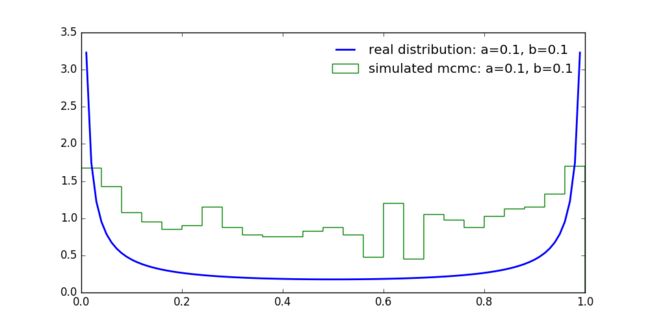
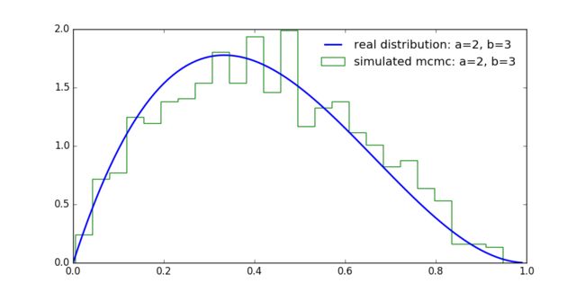
用MCMC采样算法实现对Beta 分布的采样

关于Beta distribution更详尽的内容请参见 Beta函数与Gamma函数及其与Beta分布的关系。已知Beta distribution的概率密度函数（pdf）为：

f(x;a,b)==constant⋅xα−1(1−x)β−1xα−1(1−x)β−1B(a,b)

我们假设任一的马尔科夫链具有 [0,1] 区间上的无限的状态，转移矩阵为 P ，满足 Pij=Pji （对称阵）。在下面的描述及实现中，其实我们并不需要关于 P 的任何信息。

1. 初始化马氏链 Initial State（初始状态） i∼U(0,1)

2. 随机在转移矩阵 P 的 第 i 行（表示从当前状态 i 出发可能到达的状态）中选择一个新的 Proposal State。简单起见我们选择 j∼U(0,1)

3. 计算接受概率（Acceptance Probability）（本质仍然是一种舍选）：
   

   αij=min{sjPjisiPij,1}
   
   有了前述的 Pij=Pji 的约束，对 αij 的定义可简化为：
   
   αij=min{sjsi,1}

其中， si=Cia−1(1−i)b−1,sj=Cja−1(1−j)b−1 ，

1. 取 u∼U(0,1) ，如果 u<αij ，则接受转移 i→j ，否则不接受

2. repeated

import numpy as np
import scipy.special as ss
import matplotlib.pyplot as plt

def beta_s(x, a, b):
    return x**(a-1)*(1-x)**(b-1)
def beta(x, a, b):
    return beta_s(x, a, b)/ss.beta(a, b)

def plot_mcmc(a, b):
    cur = np.random.rand()
    states = [cur]
    for i in range(10**5):
        next, u = np.random.rand()
        if u < np.min((beta_s(next, a, b)/beta_s(cur, a, b), 1)):
            states.append(next)
            cur = next
    x = np.arange(0, 1, .01)
    plt.figure(figsize=(10, 5))
    plt.plot(x, beta(x, a, b), lw=2, label='real dist: a={}, b={}'.format(a, b))
    plt.hist(states[-1000:], 25, normed=True, label='simu mcmc: a={}, b={}'.format(a, b))
    plt.show()

if __name__ == '__main__':
    plot_mcmc(0.1, 0.1)
    plot_mcmc(1, 1)
    plot_mcmc(2, 3)