关于savgol_filter的那些事儿
关于savgol_filter的那些事儿
- 曲线平滑
- 研究背景
- Savitzky-Golay算法
- SG算法相关推导
- scipy中的savgol_filter函数
- 实现代码(python)
- 后记
曲线平滑
作为CV小白的我,在面对复杂的数据(尤其是具有时间序列的数据)时,很简单的认为数据很美好,但面对数据集和kinect采集的数据时,还是洗洗睡吧(不,老老实实的平滑滤波吧)。虽然处理后的数据必然会失去很多信息(信息论),但谁又能保证采集的数据一定是True values呢。本着在可接受误差的基础上,开始了我的平滑预处理工作。正在做一个曲线平滑汇总,这篇博文是其中一部分,后续会持续更新。如有出错,希望指正,小白在此由衷的感谢。如有侵权还请谅解,感谢诸位!!!
研究背景
最近在看广义曲率分析(GCA)1 相关的论文,有点玄学的感觉,因为是精读+复现,有时需要对其中涉及的其他知识进行学习,所以有点慢:
- 奇异值分解(SVD) ,对动作数据进行降维;
- savgol_filter,采用Savitzky-Golay卷积平滑算法参看编程字典网站,博客1,博客2,博客3
- 分隔窗 ,通过奇异值分解U特征向量,构建数据向量基(basis): E ( t i ) = [ e 1 ( t i ) ∣ . . . ∣ e M ( t i ) ] E(t_i)=[e_1(t_i)|...|e_M(t_i)] E(ti)=[e1(ti)∣...∣eM(ti)],在阈值范围内,曲线的线性空间偏离较小,从而确定分隔窗大小。
Savitzky-Golay算法
wiki百科解释:Savitzky-Golay滤波器是一种数字滤波器,它可以应用于一组数据,以平滑数据,即在不改变信号趋势的情况下提高数据的精度。通过卷积的过程实现,即通过线性最小二乘法将相邻数据点的连续子集与一个低次多项式拟合。当数据点的间距相等时,可以找到最小二乘方程的解析解,其形式是一组可以应用于所有数据子的“卷积系数”
算法来源:Savitzky-Golay卷积平滑算法是移动平滑算法的改进。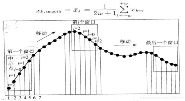
Savitzky-Golay平滑公式: x k , s m o o t h = x ‾ k = 1 H ∑ i = − w + w x k + i h i x_{k,smooth}=\overline x_k=\frac{1}{H}\sum_{i=-w}^{+w}x_{k+i}h_i xk,smooth=xk=H1i=−w∑+wxk+ihi
它使用最小二乘法将数据的一个小窗口回归到多项式上,然后使用多项式来估计窗口中心的点。其中 h i h_i hi是平滑系数,尽可能减小平滑对有用信息的影响,所以采用基于最小二乘原理,多项式拟合 h i H \frac {h_i}{H} Hhi。
应用目的:提高数据曲线的平滑性,降低噪音的干扰。
SG算法优点:在同一段曲线上,任意位置可以任意选取不同的窗宽,满足不同平滑滤波的需要;尤其是处理时序数据时,对于不同阶段的序列处理优势明显;处理non-periodic(非周期)和non-linear(非线性)来源的噪音样本效果也很好。
最小二乘法:就是"最小平方法",如有问题参看博客
SG算法相关推导
Savitzky-Golay卷积平滑关键在于矩阵算子的求解。
按照我的理解来讲:
假设我们确定滤波的window宽度是 n = 2 m + 1 n = 2m + 1 n=2m+1,则在窗口内的采样点集(samples)为 x = ( − m , − m + 1 , . . . , 0 , . . . , m − 1 , m ) x=(-m,-m+1,...,0,...,m-1,m) x=(−m,−m+1,...,0,...,m−1,m),参照图1。之后采用k-1次多项式对窗口内的数据点进行拟合。 y = a 0 + a 1 x + a 2 x 2 + . . . + a k − 1 x k − 1 y = a_0+a_1x+a_2x^2+...+a_{k-1}x^{k-1} y=a0+a1x+a2x2+...+ak−1xk−1,生成了k元线性方程组。概率论知识可知可知:若线性方程组有解,则n>k。最后通过最小二乘法拟合参数系数矩阵。
( y − m y − m + 1 ⋮ y m ) = ( 1 − m … ( − m ) k − 1 1 − m + 1 … ( − m + 1 ) k − 1 ⋮ ⋮ ⋮ ⋮ 1 m … m k − 1 ) ( a 0 a 1 ⋮ a k − 1 ) + ( e − m e − m + 1 ⋮ e m ) \begin{pmatrix} y_{-m} \\ y_{-m+1} \\ \vdots \\ y_m\end {pmatrix}= \begin{pmatrix} 1 & -m & \dots & (-m)^{k-1} \\ 1 & -m+1 & \dots & (-m+1)^{k-1} \\ \vdots & \vdots & \vdots & \vdots \\ 1 & m & \dots & m^{k-1} \end{pmatrix} \begin{pmatrix} a_{0} \\ a_{1} \\ \vdots \\ a_{k-1}\end {pmatrix}+\begin{pmatrix} e_{-m} \\ e_{-m+1} \\ \vdots \\ e_m\end {pmatrix} ⎝⎜⎜⎜⎛y−my−m+1⋮ym⎠⎟⎟⎟⎞=⎝⎜⎜⎜⎛11⋮1−m−m+1⋮m……⋮…(−m)k−1(−m+1)k−1⋮mk−1⎠⎟⎟⎟⎞⎝⎜⎜⎜⎛a0a1⋮ak−1⎠⎟⎟⎟⎞+⎝⎜⎜⎜⎛e−me−m+1⋮em⎠⎟⎟⎟⎞
矩阵表示为:
Y ( 2 m + 1 ) × 1 = X ( 2 m + 1 ) × k ⋅ A k × 1 + E ( 2 m + 1 ) × 1 Y_{(2m+1)\times1}=X_{(2m+1)\times k} \cdot A_{k \times 1}+E_{(2m+1) \times 1} Y(2m+1)×1=X(2m+1)×k⋅Ak×1+E(2m+1)×1
A A A的最小二乘解 A A A为2
A ˙ = ( X T ⋅ X ) − 1 ⋅ X T ⋅ Y \dot{A}=(X^T \cdot X)^{-1} \cdot X^T \cdot Y A˙=(XT⋅X)−1⋅XT⋅Y
Y Y Y的模型预测值或滤波值 Y ˙ \dot{Y} Y˙为
Y ˙ = X ⋅ A = X ⋅ ( X T ⋅ X ) − 1 ⋅ X T ⋅ Y = B ⋅ Y \dot{Y}=X \cdot A = X \cdot (X^T \cdot X)^{-1} \cdot X^T \cdot Y=B \cdot Y Y˙=X⋅A=X⋅(XT⋅X)−1⋅XT⋅Y=B⋅Y ⇒ B = X ⋅ ( X T ⋅ X ) − 1 ⋅ X T \Rightarrow B=X \cdot (X^T \cdot X)^{-1} \cdot X^T ⇒B=X⋅(XT⋅X)−1⋅XT
b i b_i bi是预测值模型, y i y_i yi是观测数据与 x i x_i xi无关,令 v i = y i − b i v_i=y_i-b_i vi=yi−bi, Y = ( y 1 , y 2 , . . . y n ) T Y=(y_1,y_2,...y_n)^T Y=(y1,y2,...yn)T
V = ( v 1 , v 2 , . . . , v n ) T V=(v_1,v_2,...,v_n)^T V=(v1,v2,...,vn)T V = Y − B = Y − X A V=Y-B=Y-XA V=Y−B=Y−XA Q = ∑ i r v i 2 = V T V = ( Y − X A ) T ( Y − X A ) = m i n Q=\sum_i^rv_i^2=V^TV=(Y-XA)^T(Y-XA)=min Q=i∑rvi2=VTV=(Y−XA)T(Y−XA)=min ∂ ∂ A [ ( Y − X A ) T ( Y − X A ) ] \frac{\partial}{\partial A}[(Y-XA)^T(Y-XA)] ∂A∂[(Y−XA)T(Y−XA)] ∂ ∂ A [ ( Y − X A ) T ( Y − X A ) ] = 2 ∂ ( Y − X A ) T ∂ A ( Y − X A ) = 2 ∂ ( Y T − A T X T ) ∂ A ( Y − X A ) = 2 [ ∂ Y T ∂ A − ∂ ( A T X T ) ∂ A ] ( Y − X A ) = − 2 X T ( Y − X A ) = − 2 X T Y + 2 X T X A = 0 \begin{aligned} \frac{\partial}{\partial A}[(Y-XA)^T(Y-XA)] &=2\frac{\partial(Y-XA)^T}{\partial A}(Y-XA)\\ &= 2\frac{\partial(Y^T-A^TX^T)}{\partial A}(Y-XA)\\ &= 2[\frac{\partial Y^T}{\partial A}-\frac{\partial (A^TX^T)}{\partial A}](Y-XA)\\ &=-2X^T(Y-XA)\\ &=-2X^TY+2X^TXA=0 \end{aligned} ∂A∂[(Y−XA)T(Y−XA)]=2∂A∂(Y−XA)T(Y−XA)=2∂A∂(YT−ATXT)(Y−XA)=2[∂A∂YT−∂A∂(ATXT)](Y−XA)=−2XT(Y−XA)=−2XTY+2XTXA=0 A = ( X − 1 ( X T ) − 1 X T Y ) = ( X T X ) − 1 X T Y A=(X^{-1}(X^T)^{-1}X^TY)=(X^TX)^{-1}X^TY A=(X−1(XT)−1XTY)=(XTX)−1XTY
具体几处细节看链接2。
scipy中的savgol_filter函数
官方帮助文档,解决方法简单,参数一般是(data, window_length, polynomial order)。
Parameters:
x : array_like

The data to be filtered. If x is not a single or double precision floating point array, it will be converted to type numpy.float64 before filtering.

window_length : int

The length of the filter window (i.e. the number of coefficients). window_length must be a positive odd integer.

polyorder : int

The order of the polynomial used to fit the samples. polyorder must be less than window_length.

deriv : int, optional

The order of the derivative to compute. This must be a nonnegative integer. The default is 0, which means to filter the data without differentiating.

delta : float, optional

The spacing of the samples to which the filter will be applied. This is only used if deriv > 0. Default is 1.0.

axis : int, optional

The axis of the array x along which the filter is to be applied. Default is -1.

mode : str, optional

Must be ‘mirror’, ‘constant’, ‘nearest’, ‘wrap’ or ‘interp’. This determines the type of extension to use for the padded signal to which the filter is applied. When mode is ‘constant’, the padding value is given by cval. See the Notes for more details on ‘mirror’, ‘constant’, ‘wrap’, and ‘nearest’. When the ‘interp’ mode is selected (the default), no extension is used. Instead, a degree polyorder polynomial is fit to the last window_length values of the edges, and this polynomial is used to evaluate the last window_length // 2 output values.

cval : scalar, optional

Value to fill past the edges of the input if mode is ‘constant’. Default is 0.0.

Returns:
y : ndarray, same shape as x

The filtered data.
实现代码(python)
代码学习其他博客和相关程序学习网站,侵权即删。
简单的正弦曲线平滑代码,运用scipy中的savgol_filter函数,绿色为SG平滑后曲线.
import numpy as np
import matplotlib.pyplot as plt
from scipy.signal import savgol_filter
# SG算法
x = np.linspace(0,2*np.pi,100)
y = np.sin(x) + np.random.random(100) * 0.2
yhat = savgol_filter(y, 51, 3) # window size 51, polynomial order 3
plt.plot(x,y)
plt.plot(x,yhat, color='red')
plt.show()
# 移动平均框(普通卷积法)
import numpy as np
import matplotlib.pyplot as plt
from scipy.signal import savgol_filter
# SG算法
x = np.linspace(0,2*np.pi,100)
y = np.sin(x) + np.random.random(100) * 0.2
yhat = savgol_filter(y, 51, 3) # window size 51, polynomial order 3
plt.plot(x,y)
plt.plot(x,yhat, color='red')
plt.show()
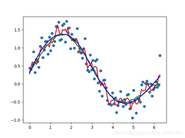
# 移动平均框(普通卷积法) + SG对比
x = np.linspace(0,2*np.pi,100)
y = np.sin(x) + np.random.random(100) * 0.8
def smooth(y, box_pts):
box = np.ones(box_pts)/box_pts
y_smooth = np.convolve(y, box, mode='same')
return y_smooth
plt.plot(x, y,'o')
plt.plot(x, smooth(y,3), 'r-', lw=2)
plt.plot(x, smooth(y,19), 'g-', lw=2)
plt.plot(x,savgol_filter(y, 51, 3), 'b-', lw=2)# window size 51, polynomial order 3
plt.show()
后记
图示不能自动编号和显示,还是我操作不对,希望指正,在这只能手敲了,如果确实没有,希望CSDN能够解决这个问题。码字不易,不喜勿喷。
1
2
Arn R T, Narayana P, Emerson T, et al. Motion segmentation via generalized curvatures[J]. IEEE transactions on pattern analysis and machine intelligence, 2018, 41(12): 2919-2932. ↩︎
矩阵的最小二乘法求解,残差平方和最小 ↩︎ ↩︎