python计算机视觉作业2

hello，大家好，博主又来了。这次给大家跑一跑python计算机视觉这本书的第二章代码。
1、SIFT特征匹配原理描述
尺度不变特征变换（Scale Invariant Feature Transform，SIFT）是David G Lowe 在1999年提出的基于不变量描述子的匹配算法，SIFT 具有以下特征：（1）SIFT特征是图像的局部特征，对平移、旋转、尺度缩放、亮度变化、遮挡和噪声等具有良好的不变性，对视觉变化、 仿射变换也保持一定程度的稳定性；（2）独特性好，信息量丰富，适用于在海量特征数据库中进行快速、准确的匹配；（3）多量性，即使少数的几个物体也可以产生大量SIFT特征向量；（4）速度相对较快，经优化的SIFT匹配算法甚至可以达到实时的要求。

SIFT特征匹配算法主要包括两个阶段，一个是SIFT特征向量的生成，第二阶段是SIFT特征向量的匹配。
1 SIFT特征向量的生成

1.1 构建尺度空间，检测极值点
由于Koendetink证明了高斯核是实现尺度变换的唯一变换核，所以对图像在不同尺度下提取图像特征，从而达到了尺度不变性。首先建立高斯金字塔，然后再建立DOG（Difference Of Gaussian）金字塔，最后在DOG金字塔的基础上进行极值检测。

1.2特征点过滤及精确定位
关键点的选取要经过两步：①它必须去除低对比度和对噪声敏感的候选关键点；②去除边缘点。

1.3为关键点分配方向值

利用特征点领域像素的梯度方向分布特征来定关键点的方向，公式如下：
（11）

（12）

m(x,y) 表示(x,y)处梯度的模值，θ(x,y)表示方向，L是关键点所在的空间尺度函数。用梯度直方图来统计邻域像素的梯度方向，如图4所示，梯度直方图的横轴代表了邻域像素的梯度方向的大小，纵轴代表了邻域像素梯度值的大小。梯度直方图的横轴的取值范围是0°~360°，每10°为一个单位。总共有36个单位。梯度方向的直方图的主峰值则代表了该关键点的主方向，如果有相当于主峰值的80%大小的其他峰值，则为该关键点的辅方向。可以看出关键点的方向就由一个主峰值方向和多个次峰值的方向决定。这样可以减少图像旋转对特征关键点的影响。

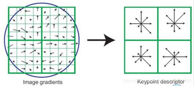
1.4生成特征向量描述子

为了进一步描述关键点的信息，则确定关键点的邻域范围的大小很重要。 如图5所示：每个小方格代表的是关键的邻域像素，小方格内的的箭头代表了该邻域像素的梯度方向，箭头的大小代表了梯度大小。图5(b)中的左上角的小方块由图5(a)中的左上角的四个小方格组成。即：（b）图中的每个小方块的方向是对于（a）图中的方格方向的累积值。 图5显示的是（a）图是8×8的邻域范围，（b）图显示的是 2×2 的种子点（每个方格代表一个种子）。 为了增强抗噪能力和匹配的稳健性，通常把邻域的取值范围设成16×16，那么就会产生 4×4 的种子点。 这样每个关键点的信息量就包含在了4×4×8=128维特征向量里。

2 SIFT特征向量的匹配

对SIFT特征向量进行匹配是根据相似性度量来进行的，常用的匹配方法有：欧式距离和马氏距离等。采用欧氏距离对SIFT的特征向量进行匹配。获取SIFT特征向量后, 采用优先k-d树进行优先搜索来查找每个特征点的近似最近邻特征点。在这两个特征点中，如果最近的距离除以次近的距离少于某个比例阈值，则接受这一对匹配点。降低这个比例阈值， SIFT匹配点数目会减少，但更加稳定。

2、Harris算法对图像进行特征匹配，代码如下：

 # -*- coding: utf-8 -*-
from pylab import *
from PIL import Image

from PCV.localdescriptors import harris
from PCV.tools.imtools import imresize

"""
This is the Harris point matching example in Figure 2-2.
"""

# Figure 2-2上面的图
#im1 = array(Image.open("../data/crans_1_small.jpg").convert("L"))
#im2= array(Image.open("../data/crans_2_small.jpg").convert("L"))

# Figure 2-2下面的图
im1 = array(Image.open("library1.jpg").convert("L"))
im2 = array(Image.open("library2.jpg").convert("L"))

# resize加快匹配速度
im1 = imresize(im1, (im1.shape[1]/2, im1.shape[0]/2))
im2 = imresize(im2, (im2.shape[1]/2, im2.shape[0]/2))

wid = 5
harrisim = harris.compute_harris_response(im1, 5)
filtered_coords1 = harris.get_harris_points(harrisim, wid+1)
d1 = harris.get_descriptors(im1, filtered_coords1, wid)

harrisim = harris.compute_harris_response(im2, 5)
filtered_coords2 = harris.get_harris_points(harrisim, wid+1)
d2 = harris.get_descriptors(im2, filtered_coords2, wid)

print 'starting matching'
matches = harris.match_twosided(d1, d2)

figure()
gray()
harris.plot_matches(im1, im2, filtered_coords1, filtered_coords2, matches)
show()

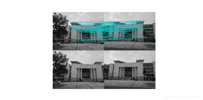
正如你从上图所看到的，这里有很多错配的。近年来，提高特征描述点检测与描述有了很大的发展，下面博主将会带大家展示特征匹配最好的算法之一——SIFT
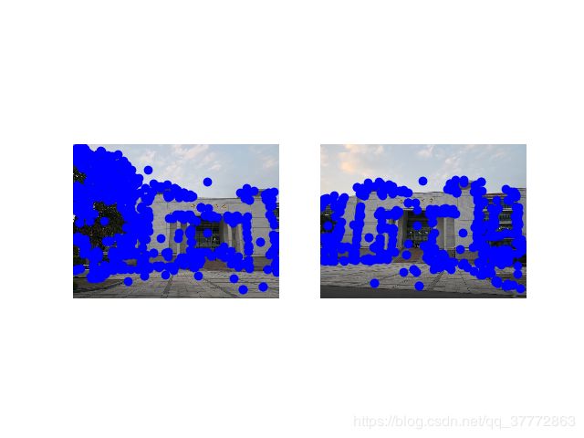
3、SIFT算法对图像进行特征匹配，代码如下：

from PIL import Image
from pylab import *
import sys
from PCV.localdescriptors import sift


if len(sys.argv) >= 3:
  im1f, im2f = sys.argv[1], sys.argv[2]
else:
#  im1f = '../data/sf_view1.jpg'
#  im2f = '../data/sf_view2.jpg'
  im1f = 'library1.jpg'
  im2f = 'library2.jpg'
#  im1f = '../data/climbing_1_small.jpg'
#  im2f = '../data/climbing_2_small.jpg'
im1 = array(Image.open(im1f))
im2 = array(Image.open(im2f))

sift.process_image(im1f, 'out_sift_1.txt')
l1, d1 = sift.read_features_from_file('out_sift_1.txt')
figure()
gray()
subplot(121)
sift.plot_features(im1, l1, circle=False)

sift.process_image(im2f, 'out_sift_2.txt')
l2, d2 = sift.read_features_from_file('out_sift_2.txt')
subplot(122)
sift.plot_features(im2, l2, circle=False)

#matches = sift.match(d1, d2)
matches = sift.match_twosided(d1, d2)
print '{} matches'.format(len(matches.nonzero()[0]))

figure()
gray()
sift.plot_matches(im1, im2, l1, l2, matches, show_below=True)
show()
print'matching done!'

运行上面代码，可得到下图：


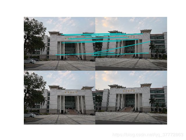
4、sift和harris特征点匹配实验结果的对比
　从理论上说，SIFT是一种相似不变量，即对图像尺度变化和旋转是不变量。然而，由于构造SIFT特征时，在很多细节上进行了特殊处理，使得SIFT对图像的复杂变形和光照变化具有了较强的适应性，同时运算速度比较快，定位精度比较高。
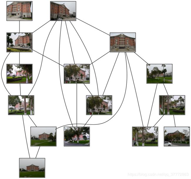
　5、匹配地理标记图像
　下面将使用局部描述算子来匹配带有地理标记的图像，代码如下：

# -*- coding: utf-8 -*-
from pylab import *
from PIL import Image
from PCV.localdescriptors import sift
from PCV.tools import imtools
import pydot

""" This is the example graph illustration of matching images from Figure 2-10.
To download the images, see ch2_download_panoramio.py."""

#download_path = "panoimages"  # set this to the path where you downloaded the panoramio images
#path = "/FULLPATH/panoimages/"  # path to save thumbnails (pydot needs the full system path)

download_path = "F:/dropbox/Dropbox/translation/pcv-notebook/data/panoimages"  # set this to the path where you downloaded the panoramio images
path = "F:/dropbox/Dropbox/translation/pcv-notebook/data/panoimages/"  # path to save thumbnails (pydot needs the full system path)

# list of downloaded filenames
imlist = imtools.get_imlist(download_path)
nbr_images = len(imlist)

# extract features
featlist = [imname[:-3] + 'sift' for imname in imlist]
for i, imname in enumerate(imlist):
    sift.process_image(imname, featlist[i])

matchscores = zeros((nbr_images, nbr_images))

for i in range(nbr_images):
    for j in range(i, nbr_images):  # only compute upper triangle
        print 'comparing ', imlist[i], imlist[j]
        l1, d1 = sift.read_features_from_file(featlist[i])
        l2, d2 = sift.read_features_from_file(featlist[j])
        matches = sift.match_twosided(d1, d2)
        nbr_matches = sum(matches > 0)
        print 'number of matches = ', nbr_matches
        matchscores[i, j] = nbr_matches
print "The match scores is: \n", matchscores

# copy values
for i in range(nbr_images):
    for j in range(i + 1, nbr_images):  # no need to copy diagonal
        matchscores[j, i] = matchscores[i, j]

#可视化

threshold = 2  # min number of matches needed to create link

g = pydot.Dot(graph_type='graph')  # don't want the default directed graph

for i in range(nbr_images):
    for j in range(i + 1, nbr_images):
        if matchscores[i, j] > threshold:
            # first image in pair
            im = Image.open(imlist[i])
            im.thumbnail((100, 100))
            filename = path + str(i) + '.png'
            im.save(filename)  # need temporary files of the right size
            g.add_node(pydot.Node(str(i), fontcolor='transparent', shape='rectangle', image=filename))

            # second image in pair
            im = Image.open(imlist[j])
            im.thumbnail((100, 100))
            filename = path + str(j) + '.png'
            im.save(filename)  # need temporary files of the right size
            g.add_node(pydot.Node(str(j), fontcolor='transparent', shape='rectangle', image=filename))

            g.add_edge(pydot.Edge(str(i), str(j)))
g.write_png('whitehouse.png')

实验结果如下：

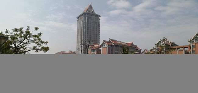
最后，博主配上一张集美大学的风景图，hhh

谢谢阅读！