【NLP】卷积神经网络基础

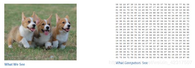
The role of the ConvNet is to reduce the images into a form which is easier to process, without losing features which are critical for getting a good prediction.

我们今天就大概看三种layers：convolution Layer , pooling layer 和 fully connected layer.

1. Convolution Layer

1.1 Parameters:

Kernel Size, Stride, Padding, Input & Output Channels

- Kernel/Filter

如上动图：Kernel/Filter在这里是个3x3x1 matrix，每个channel选的kernel都不一样

Kernel/Filter, K = 
1  0  0
1  -1  -1
1  0  -1

卷积核大小：
卷积核通常使用奇数 3*3, 55, 77, 9*9, （为了对称）
通常小而深

- Stride

楼上kernel的Stride Length = 1 (Non-Strided)，如果是stride=2的就如下图：
（蓝色的表示input，阴影是kernel，青色的表示output）

- Padding

还有各种带padding的示意图，看这里here

a) Same Padding

（图：SAME padding: 5x5x1 image is padded with 0s to create a 6x6x1 image）

When we augment the 5x5x1 image into a 6x6x1 image and then apply the 3x3x1 kernel over it, we find that the convolved matrix turns out to be of dimensions 5x5x1. Hence the name — Same Padding.

b) Valid Padding

Iif we perform the same operation without padding, we are presented with a matrix which has dimensions of the Kernel (3x3x1) itself — Valid Padding.

1.2 Do the math:

· multiply, then add up：

简单来讲，看下图，黄的里面每一个格子和对应绿色里面的格子相乘，然后相加，得到的就就是Convolved feature

（图：Convoluting a 5x5x1 image with a 3x3x1 kernel to get a 3x3x1 convolved feature）
详细的见本页2.2 Convolution Matrix.

2. Transposed Convolutions

也叫 deconvolutions 或者 fractionally strided convolutions
对叫作deconvolution抱有怨念大有人在，如图：

为啥叫deconvolution，请找 Zeiler.

2.1 why use?

the need of up-sampling, 譬如从低像素到高像素，使用Transposed Convolutions就是个很好的办法。

参考

2.2 Intuition:

- Convolution Operation

回顾一下卷积运算：

input: 4x4 
stride: 1
kernel: 3x3
padding: 无
output: 2x2 

这里，9个数变1个数，卷积运算是多对一的关系。

- Going Backward

如果我们想：

input: 2x2 
output: 4x4 

也就是1个数变成9个数，一对多的关系。
我们首先需要弄明白Convolution Matrix和Transposed Convolution Matrix：

- Convolution Matrix

如下图，把 3x3 kernel变成4x16 matrix，把 4x4 input matrix变成16x1的column vector，
然后将 4x16 convolution matrix 与 16x1 input matrix (16 dimensional column vector)矩阵相乘，得到4x1 matrix

4x1 matrix进行变换就是2x2 matrix ：

为啥要弄成Convolution Matrix？
With the convolution matrix, you can go from 16 (4x4) to 4 (2x2) because the convolution matrix is 4x16. Then, if you have a 16x4 matrix, you can go from 4 (2x2) to 16 (4x4).

- Transposed Convolution Matrix

我们若想：

input: 2x2 
output: 4x4 

我们要用到 16x4 matrix，这里要保证 1个数对应9个数的关系:

• Transpose the convolution matrix C (4x16) to C^T (16x4).
• Matrix-multiply C^T (16x4) with a column vector (4x1) to generate an output matrix (16x1)
• The transposed matrix connects 1 value to 9 values in the output.
  
  把结果变形就得到了4x4 matrix：
  

注意：the actual weight values in the matrix does not have to come from the original convolution matrix. What’s important is that the weight layout is transposed from that of the convolution matrix. here

tensorflow

tf.nn.conv2d_transpose(
    value,
    filter, 
    output_shape,
    strides,
    padding='SAME', 
    data_format='NHWC',
    name=None
)

3. Pooling Layer

In all cases, pooling helps to make the representation become approximately invariant to small translations of the input. Invariance to translation means that if we translate the input by a small amount, the values of most of the pooled outputs do not change. — Page 342, Deep Learning, 2016.

说白了就是化繁为简，等于downsampling：

作用1: decrease the computational power required to process the data through dimensionality reduction.
作用2: useful for extracting dominant features which are rotational and positional invariant, thus maintaining the process of effectively training of the model.

两种pooling：

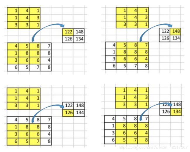
3.1 Max pooling

字面意思，max()，如图

3.2 Average pooling

字面意思，average()，如图

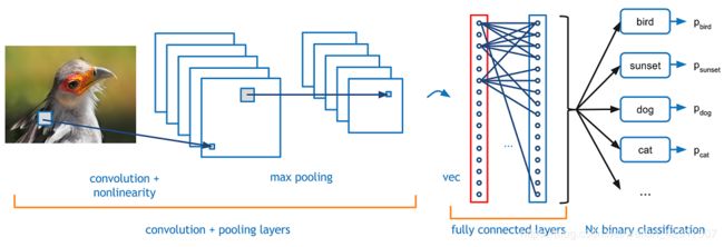
4. Fully Connected Layer

Basically, a FC layer looks at what high level features most strongly correlate to a particular class and has particular weights so that when you compute the products between the weights and the previous layer, you get the correct probabilities for the different classes.

5. CNN Architectures

参考

5.1 Classic network architectures

- LeNet-5

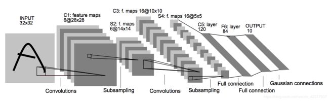
看这里：Gradient-based learning applied to document recognition

- AlexNet

看这里：ImageNet Classification with Deep Convolutional Neural Networks

- VGG 16

看这里：Very Deep Convolutional Networks for Large-Scale Image Recognition

5.2 Modern network architectures

- Inception(GoogLeNet)

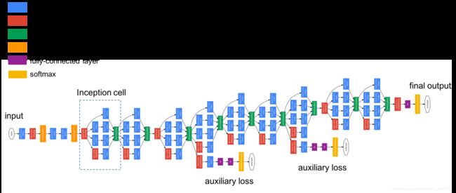
看这里: Going deeper with convolutions

- ResNet

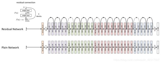
看这里：Deep Residual Learning for Image Recognition

- ResNeXt

看这里：Aggregated Residual Transformations for Deep Neural Networks

- DenseNet

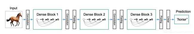
看这里：Densely Connected Convolutional Networks

6. Text-CNN

参考

7. Implementing a CNN for Text Classification in TensorFlow

参考here

import tensorflow as tf
import numpy as np
 
class TextCNN(object):
    """
    A CNN for text classification.
    Uses an embedding layer, followed by a convolutional, max-pooling and softmax layer.
   """
    def __init__(
      self, sequence_length, num_classes, vocab_size,
      embedding_size, filter_sizes, num_filters):
        # Implementation...

Arguments:

• sequence_length – The length of our sentences. Remember that we padded all our sentences to have the same length (59 for our data set).
• num_classes – Number of classes in the output layer, two in our case (positive and negative).
• vocab_size – The size of our vocabulary. This is needed to define the size of our embedding layer, which will have shape [vocabulary_size, embedding_size].
• embedding_size – The dimensionality of our embeddings.
• filter_sizes – The number of words we want our convolutional filters to cover. We will have num_filters for each size specified here. For example, [3, 4, 5] means that we will have filters that slide over 3, 4 and 5 words respectively, for a total of 3 * num_filters filters.
• num_filters – The number of filters per filter size (see above).

# Placeholders for input, output and dropout
self.input_x = tf.placeholder(tf.int32, [None, sequence_length], name='input_x')
self.input_y = tf.placeholder(tf.float32, [None, num_classes], name='input_y')
self.dropout_keep_prob = tf.placeholder(tf.float32, name='dropout_keep_prob')

#embedding layer
with tf.device('/cpu:0'), tf.name_scope('embedding'):
    W = tf.Variable(
        tf.random_uniform([vocab_size, embedding_size], -1.0, 1.0),
        name='W')
    self.embedded_chars = tf.nn.embedding_lookup(W, self.input_x)
    self.embedded_chars_expanded = tf.expand_dims(self.embedded_chars, -1)
#Convolution and Max-Pooling Layers
pooled_outputs = []
for i, filter_size in enumerate(filter_sizes):
    with tf.name_scope('conv-maxpool-%s' % filter_size):
        # Convolution Layer
        filter_shape = [filter_size, embedding_size, 1, num_filters]
        W = tf.Variable(tf.truncated_normal(filter_shape, stddev=0.1), name='W')
        b = tf.Variable(tf.constant(0.1, shape=[num_filters]), name='b')
        conv = tf.nn.conv2d(
            self.embedded_chars_expanded,
            W,
            strides=[1, 1, 1, 1],
            padding='VALID',
            name='conv')
        # Apply nonlinearity
        h = tf.nn.relu(tf.nn.bias_add(conv, b), name='relu')
        # Max-pooling over the outputs
        pooled = tf.nn.max_pool(
            h,
            ksize=[1, sequence_length - filter_size + 1, 1, 1],
            strides=[1, 1, 1, 1],
            padding='VALID',
            name='pool')
        pooled_outputs.append(pooled)
 
# Combine all the pooled features
num_filters_total = num_filters * len(filter_sizes)
self.h_pool = tf.concat(3, pooled_outputs)
self.h_pool_flat = tf.reshape(self.h_pool, [-1, num_filters_total])


# Add dropout layer
with tf.name_scope('dropout'):
    self.h_drop = tf.nn.dropout(self.h_pool_flat, self.dropout_keep_prob)
    
##scores and prediction
with tf.name_scope('output'):
    W = tf.Variable(tf.truncated_normal([num_filters_total, num_classes], stddev=0.1), name='W')
    b = tf.Variable(tf.constant(0.1, shape=[num_classes]), name='b')
    self.scores = tf.nn.xw_plus_b(self.h_drop, W, b, name='scores')
    self.predictions = tf.argmax(self.scores, 1, name='predictions')

# Calculate mean cross-entropy loss
with tf.name_scope('loss'):
    losses = tf.nn.softmax_cross_entropy_with_logits(self.scores, self.input_y)
    self.loss = tf.reduce_mean(losses)
    
# Calculate Accuracy
with tf.name_scope('accuracy'):
    correct_predictions = tf.equal(self.predictions, tf.argmax(self.input_y, 1))
    self.accuracy = tf.reduce_mean(tf.cast(correct_predictions, 'float'), name='accuracy')
    
#Training Procedure 
with tf.Graph().as_default():
    session_conf = tf.ConfigProto(
      allow_soft_placement=FLAGS.allow_soft_placement,
      log_device_placement=FLAGS.log_device_placement)
    sess = tf.Session(config=session_conf)
    with sess.as_default():
        # Code that operates on the default graph and session comes here..

#Instantiating the CNN and minimizing the loss

cnn = TextCNN(
    sequence_length=x_train.shape[1],
    num_classes=2,
    vocab_size=len(vocabulary),
    embedding_size=FLAGS.embedding_dim,
    filter_sizes=map(int, FLAGS.filter_sizes.split(',')),
    num_filters=FLAGS.num_filters)
    
global_step = tf.Variable(0, name='global_step', trainable=False)
optimizer = tf.train.AdamOptimizer(1e-4)
grads_and_vars = optimizer.compute_gradients(cnn.loss)
train_op = optimizer.apply_gradients(grads_and_vars, global_step=global_step)


# Output directory for models and summaries
timestamp = str(int(time.time()))
out_dir = os.path.abspath(os.path.join(os.path.curdir, 'runs', timestamp))
print('Writing to {}\n'.format(out_dir))
 
# Summaries for loss and accuracy
loss_summary = tf.scalar_summary('loss', cnn.loss)
acc_summary = tf.scalar_summary('accuracy', cnn.accuracy)
 
# Train Summaries
train_summary_op = tf.merge_summary([loss_summary, acc_summary])
train_summary_dir = os.path.join(out_dir, 'summaries', 'train')
train_summary_writer = tf.train.SummaryWriter(train_summary_dir, sess.graph_def)
 
# Dev summaries
dev_summary_op = tf.merge_summary([loss_summary, acc_summary])
dev_summary_dir = os.path.join(out_dir, 'summaries', 'dev')
dev_summary_writer = tf.train.SummaryWriter(dev_summary_dir, sess.graph_def)

# Checkpointing
checkpoint_dir = os.path.abspath(os.path.join(out_dir, 'checkpoints'))
checkpoint_prefix = os.path.join(checkpoint_dir, 'model')
# Tensorflow assumes this directory already exists so we need to create it
if not os.path.exists(checkpoint_dir):
    os.makedirs(checkpoint_dir)
saver = tf.train.Saver(tf.all_variables())

#Initializing the variables
sess.run(tf.initialize_all_variables())

#define a function for a single training step, evaluating the model on a batch of data and updating the model parameters.
def train_step(x_batch, y_batch):
    '''
    A single training step
    '''
    feed_dict = {
      cnn.input_x: x_batch,
      cnn.input_y: y_batch,
      cnn.dropout_keep_prob: FLAGS.dropout_keep_prob
    }
    _, step, summaries, loss, accuracy = sess.run(
        [train_op, global_step, train_summary_op, cnn.loss, cnn.accuracy],
        feed_dict)
    time_str = datetime.datetime.now().isoformat()
    print('{}: step {}, loss {:g}, acc {:g}'.format(time_str, step, loss, accuracy))
    train_summary_writer.add_summary(summaries, step)
    
#print the loss and accuracy of the current training batch and save the summaries to disk

def dev_step(x_batch, y_batch, writer=None):
    '''
    Evaluates model on a dev set
    '''
    feed_dict = {
      cnn.input_x: x_batch,
      cnn.input_y: y_batch,
      cnn.dropout_keep_prob: 1.0
    }
    step, summaries, loss, accuracy = sess.run(
        [global_step, dev_summary_op, cnn.loss, cnn.accuracy],
        feed_dict)
    time_str = datetime.datetime.now().isoformat()
    print('{}: step {}, loss {:g}, acc {:g}'.format(time_str, step, loss, accuracy))
    if writer:
        writer.add_summary(summaries, step)
        
# Training Loop
# Generate batches
batches = data_helpers.batch_iter(
    zip(x_train, y_train), FLAGS.batch_size, FLAGS.num_epochs)
# Training loop. For each batch...
for batch in batches:
    x_batch, y_batch = zip(*batch)
    train_step(x_batch, y_batch)
    current_step = tf.train.global_step(sess, global_step)
    if current_step % FLAGS.evaluate_every == 0:
        print('\nEvaluation:')
        dev_step(x_dev, y_dev, writer=dev_summary_writer)
        print('')
    if current_step % FLAGS.checkpoint_every == 0:
        path = saver.save(sess, checkpoint_prefix, global_step=current_step)
        print('Saved model checkpoint to {}\n'.format(path))