数据分析实例1（英文报告）--预测未来收入--SAS 逻辑回归--1994年美国人口普查数据

Prediction of Future Income by Using Logistic Regression

Matthew LaFrance， Yu Zhang

 

1 Introduction

Many factors could influence a person’s annual income, for example, age, gender, race, level of education, marriage status, nationality, etc. The authors tried to fit four models of influential factors that based on a census dataset and to find a precise prediction of annual income.

The dataset was found at the UCI Machine Learning Repository. The data consists of 48,844 observations from a 1994 U.S. Census. The target variable, “Salary”, has two levels: >50k and <=50k. There are 8 categorical features and 5
numeric features consisting of demographic, educational, and occupational information. Table 1 is the variables in SAS version.
 

Table 1 Variables in the Income Dataset

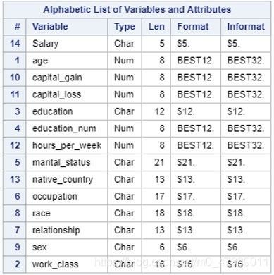
The target variable “Salary” is notably unbalanced (in table 2). As a result, we noted that using raw accuracy as a success metric could potentially be misleading because a model that classifies all observations as <=50k would achieve roughly 76% accuracy.
 
Table 2 Salary Overview

2 Data Preprocessing

2.1 Missing Values

3,622 observations contained missing values primarily in the “occupation” column. Because the occupation column had many factor levels, we decided many imputation methods wouldn’t retain enough information to justify the increase in bias, so we decided to take only complete cases. As a result, our conclusions may be biased, and we assume that the deleted observations had missing values at random. For future work, it may be worthwhile to explore other methods of handling the missing data. After deletion, the final dataset had 45,222 observations.
 

2.2 Multicollinearity Checks

None of our numeric features showed strong correlations between each other (see table 3). As a result, we were not particularly concerned about multicollinearity.
 

Table 3 The Result of Correlation Checks

2.3 Exploratory Data Analysis and Feature Engineering

In our initial looks at the data, we were able to make several noteworthy observations which will be detailed below by variables and summarized at the end.

2.3.1 Capital Gains and Capital Losses

Figure 1 Overview of Capital Gains

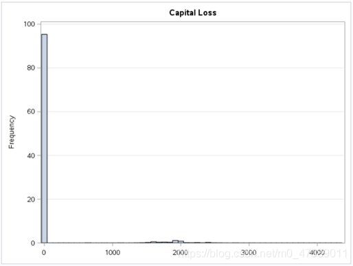
Figure 2 Overview of Capital Losses
 

Regarding the capital gains and loss variables, it is worth noting that most individuals in our dataset do not have any investments (see Figure 1 and Figure 2).

2.3.2 Native Country
As expected, most observations are U.S. natives (see Figure 3). The native country variable consists of many factor levels. In order to avoid having too many dummy variables later on, we decided it would be necessary to rebin this feature into a “0, and 1 ” indicator variable of being a native-born citizen.

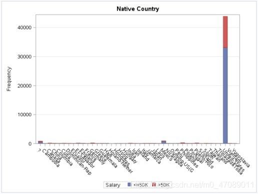
Figure 3 Overview of Native Countries
 

2.3.3 Marital Status
In looking into the marital status feature, we noticed several different levels all representing married (see Figure 4). We decided to combine all these levels into one level, “married”, for more convenient interpretation. Additionally, it was worth noting that married individuals appear to more consistently make greater than 50k.

Figure 4 Overview of Marital Status
 

2.3.4 Education Level
As expected with education, it appears that individuals who complete higher education tend to make more than 50k than others (see Figure 5). In our dataset we had two variables that represented education categorically and numerically. In the end, we decided to drop the categorical version and only include the variable “education_num” in the final model. This factor consists of the number of years of school completed by each observation and offers the same information in more easily interpretable format.

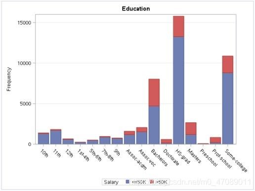
Figure 5 Overview of Education Level

In summary, we have four approaches of feature engineering. The first, we rebinned all marital status levels that contain “married…” to “married”. The second, we changed “native_country” to a “0, and 1” indicator of U.S. native or not U.S. native. The third, we combined occupation levels “Armed Forces” with “Protective Services”. The forth, we dropped categorical education variable in favor of the numeric version.
 

3 Modelling

We fitted a total of four models in this project. Our primary model was a logistic regression model with all variables included. Additionally, we fit a decision tree, random forest, and gradient tree boosting model. All three of the latter models outperformed the logistic regression in terms of accuracy and AUC score, but the logistic performed reasonably well and provided the most easily interpretable results.

3.1 Logistic Regression

The Binary Logistic Regression Model is classification method where a binary response variable is related to a set of categorical or numeric features. Whereas linear regression models the expected value of the response variable, logistic regression models the predicted probability of the response taking a specific value.

3.1.1 Model Fitting
First, we randomly split the whole dataset to the training dataset and the test dataset by 1/3 to 2/3. The we fit an initial model with all variables included in SAS using proc logistic. To assess the fit, we constructed a calibration plot, see Figure 6.

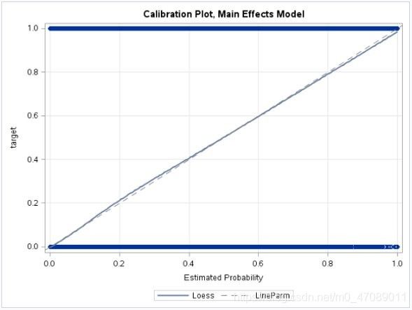
Figure 6 Calibration Plot of Logistic Regression

Based on this plot (Figure 6) the fit appeared to be good. Additionally, the model passed the global hypothesis tests of H0: Beta=0.
 

Table 4 The Results of Hypothesis Test

As a final check, we decided to perform a Homser-Lemeshow Goodness-of-Fit Test which is failed.
 

Table 5 The Result of Homser-Lemeshow Goodness-of-Fit Test

This result prompted us to consider a “probit” link function instead.
 

Table 6 The Result of Homser-Lemeshow Goodness-of-Fit Test with “probit” Link

Though the Hosmer-Lemeshow Test indicated that the “probit” link function provided a better fit, we decided to proceed using the logit link. In comparing model performance, the logit and probit models both gave essentially the same predictions and conclusions. Due to this fact we favored the logit model due to its more easily interpreted results.

3.1.2 Variable Selection
In this initial model, all features showed significant results. In order to check if we could proceed with a smaller pool of variables we performed backwards on this model. In doing so, all variables were still included in the final model. In order to gain a broader picture of this process we bootstrapped the variable selection process and performed 100 runs of it. Through this method we can check the stability of the variable selection process.
 
Table 7 The Results of Bootstrapped Variable Selection

This result showed that all factors were almost always included across all bootstrap samples. As a result, we were able to more confidently include all variables in our final model.

3.1.3 Model Performance
To asses our model’s performance we did a simple two-fold cross validation. The model performed reasonably well on both our training and test sets (see Figure 7 and Figure 8). As a result, we felt confident that our model was not simply overfitting and that it would likely be fit for use on new data.

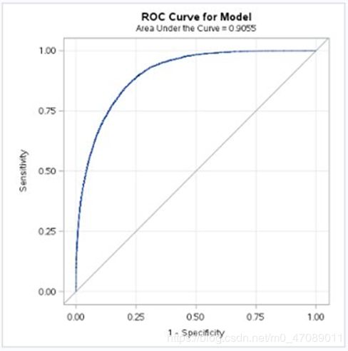
Figure 7 The ROC Curve of Model

Figure 8 ROC Curve for test Data
 

3.1.4 Parameter Estimates and Interpretations

Table 8 The Results of Maximum Likelihood Estimates

Table 9 The Results of Odds Ratio

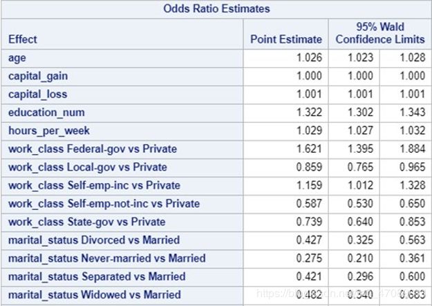
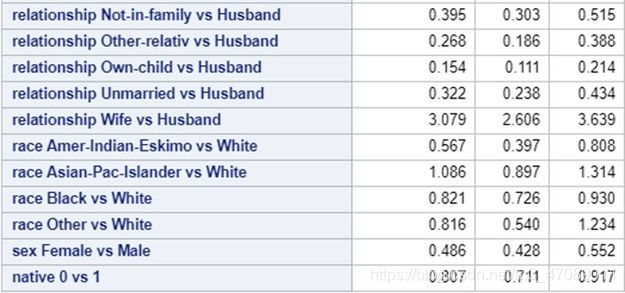
Based on the results of MLE and odds ratio in Table 8 and Table 9, we could interpret the model in the ways below.

Age: for each additional year of age there is an expected 3% increase in the odds of making >50k. This is not surprising given that with age comes experience and additional training and skills which would lead to more earning potential.

Investments: both capital gains and loss show positive relationships. Though it is intuitive that capital gains would have a positive coefficient, it is not as obvious that capital losses would. Capital losses represents any loss of income from an investment decreasing in value. Perhaps the coefficient is positive because it represents the presence of investment rather than loss of income. Individuals with money to invest likely earn more than others and likely still earn more despite experiencing losses in
their investments.

Education: for each additionally year of education we would expect a 32% increase in the odds of making >50k. Further work may be necessary with this model because higher years of education likely have stronger influence than early years. It is unlikely that each additional year increases one’s odds at a flat 30% rate. However, this conclusion does support that education plays a strong role in an income class.

Work Hours: hours per week is fairly intuitive. For each additional hour of work per week we would expect a 3% increase in the odds of being in the higher income class.

Work Class: Probably the strangest result is that we would expect federal government workers to be 62% more likely to be in the upper income class than private employees. Though one would expect private industry to be the most lucrative work class, this result likely exists because our target is binary split at 50k. As a result, we would conclude that federal government is likely not the most lucrative field, but rather employees more consistently make >50k in the federal government.

Marital Status: The only marital status factor level that differs from married is never-married. Never-married individuals are expected to 70% less likely to make >50k than married individuals. Regarding this result, it is possible that marital status is acting as a surrogate for age. Younger people likely make less money and are more likely to be unmarried.

Relationship: We are unable to draw meaningful conclusions using the relationship variable. The factor levels do not give any indication of what it represents i.e. Husband vs. Only Child. Our data source does not provide documentation as to what it means either. It is included in our final model because it does improve performance. Though we were hesitant to include an apparently uninterpretable predictor, we assume it does hold some utility given that it was a worth gathering in the census.

Race: Based on our model, we would expect the odds of Asian individuals to be about 9% greater than white people to make >50k. Additionally we would expect Native Americans to be about 60% less likely to be in the upper income class.

Sex: Regarding gender, our model indicates that we would expect females to be about 50% less likely to be in the upper income class than males. This result is surprising, but it is difficult to draw any further conclusions using our data. As with all our conclusions, we would be able to draw stronger conclusions if our target variable was continuous rather than binary.

Native Status: Lastly our model indicates that the odds of non-native individuals being in the upper income class are 20% lower than the native individuals.
 

3.2 Additional Models

After our Logistic Regression provided reasonably strong results, we decided to try a
few other models to compare it against. We compared four models: Logistic Regression, Decision Tree, Random Forest, and Gradient Bossting. This process is summarized below. Each of the below models were fit in python using the sklearn package. Tuning parameters can be found in the full code at the end of the report.
 

Table 10 The Comparison of Four Models

Model	Accuracy	AUC
Logistic Regression​	0.842053​	0.901452
Decision Tree​	0.848247	0.886360​
Random Forest​	0.851897	0.908829
Gradient Boosting	0.867824 ​	0.924975​

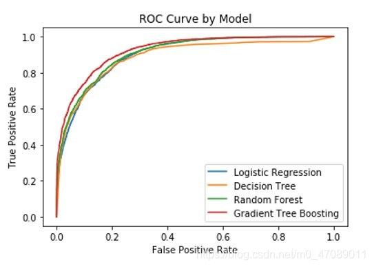
Figure 9 The ROC Curves of all Models

 

4 Conclusion

Overall, these results were not surprising. Theoretically, it is expected that a well-tuned Random Forest would be able to outperform a Logistic Regression, and the Gradient Boosting method should be able to outperform a Random Forest as well. In terms of raw predictability the Gradient Boosting model provided best results in both accuracy and AUC. Despite this the Logistic Regression model may still be preferable due to its only slightly worse performance and more interpretable results.

 

Reference

1 Agresti, Alan, Catagorical Data Analysis(3rd Edition), Wiley Series in Probability
and Statistics

2 The income dataset, Retrieved from https://archive.ics.uci.edu/ml/datasets/Adult

 

Partial SAS Code

/*Data Import*/

proc import datafile='/home/mjl16d0/Misc Data/adult.data'

            dbms=csv
out=adult1
replace;

            delimiter=',';

            getnames=no;

            datarow=1;

run;

proc import datafile='/home/mjl16d0/Misc Data/adult.test'

            dbms=csv
out=adult2
replace;

            delimiter=',';

            getnames=no;

            datarow=1;

run;

data adult2;

    set adult2;

    VAR15 = substr(VAR15,1,5);

run;

/*checking imported data*/

proc print data=adult1(obs=10);run;

proc print data=adult2(obs=10);run;

PROC CONTENTS DATA=adult1;
RUN;

PROC CONTENTS DATA=adult2;
RUN;

/*remove unnecessary . at end*/

data adult;

    set adult1 adult2;

    VAR15=compress(VAR15,'.');

run;

proc print
data=adult(firstobs=48000);run;

/*Name Variables, Drop fnlwgt (not useful)*/

data census;

    set adult(drop=var3);

    rename var1=age
var2=work_class


           var4=education
var5=education_num
var6=marital_status

           var7=occupation
var8=relationship
var9=race
var10=sex


           var11=capital_gain
var12=capital_loss

           var13=hours_per_week
var14=native_country
var15=Salary;

run;

/* Macro Variables for convenience */

%let numeric =
age capital_gain capital_loss education_num hours_per_week;

%let categoric =
work_class education marital_status occupation relationship race

                  sex native_country;

%let target =Salary;

/*Check macro vars*/

%put 'Numeric Vars:' &numeric;

%put 'Categorical Vars:' &categoric;

%put 'Target:' ⌖


/*Check distinct values of categorical data*/

proc freq data=census nlevels;

    tables Salary;

/*Plotting each feature*/

run;

proc sgplot data=census;

  title 'Age';

  histogram Age /binwidth=3;

  xaxis display=(nolabel);

  yaxis grid 
label='Frequency';

  run;

proc sgplot data=census;

  title 'Capital Gain';

  histogram capital_gain ;

  xaxis display=(nolabel);

  yaxis grid 
label='Frequency';

  run;

proc sgplot data=census;

  title 'Capital Loss';

  histogram capital_loss ;

  xaxis display=(nolabel);

  yaxis grid 
label='Frequency';

  run;

proc sgplot data=census;

  title 'Hours Per Week';

  histogram hours_per_week ;

  xaxis display=(nolabel);

  yaxis grid 
label='Frequency';

  run;

proc sgplot data=census;

  title 'Education (Numeric)';

  histogram Education_num ;

  xaxis display=(nolabel);

  yaxis grid 
label='Frequency';

  run;

proc sgplot data=census;

  title 'Work Class';

  vbar work_class /
group=Salary
stat=freq;

  xaxis display=(nolabel);

  yaxis grid 
label='Frequency';

  run;

proc sgplot data=census;

  title 'Sex';

  vbar Sex / group=Salary
stat=freq;

  xaxis display=(nolabel);

  yaxis grid 
label='Frequency';

  run;

proc sgplot data=census;

  title 'Race';

  vbar Race / group=Salary
stat=freq;

  xaxis display=(nolabel);

  yaxis grid 
label='Frequency';

  run;

proc sgplot data=census;

  title 'Education';

  vbar Education /
group=Salary
stat=freq;

  xaxis display=(nolabel);

  yaxis grid 
label='Frequency';

  run;

proc sgplot data=census;

  title 'Marital Status';

  vbar marital_status /
group=Salary
stat=freq;

  xaxis display=(nolabel);

  yaxis grid 
label='Frequency';

  run;

proc sgplot data=census;

  title 'Native Country';

  vbar native_country /
group=Salary
stat=freq;

  xaxis display=(nolabel);

  yaxis grid 
label='Frequency';

  run;

/*More Data cleaning*/

data clean;

    set census;

    /*change ?'s to blanks*/

    if work_class='?' then work_class=' '; 

    if occupation='?' then occupation= ' ';

    if native_country='?' then native_country= ' ';

    /*Create missing value flag variable*/

    /*https://communities.sas.com/t5/SAS-Procedures/Flag-Missing-Values-in-a-Dataset/td-p/200676*/

    /*This could be used if we want to try to train a classifier for random imputation.*/

    length missvar $400
hasmiss 3;

    array x{*} $ work_class occupation
native_country;

    do i=1 to dim(x);

    if missing(x{i})
then missvar=catx('_',missvar,vname(x{i}));

        end;

        drop i;

    /*Create 0,1 indicator of any missing value in an obs*/

    if missvar=' ' then hasmiss=0;

    else hasmiss=1;

run;

proc contents data=clean;run;

 

/*Create final analytic file*/

data
final;

    set clean;

    /*take only complete cases*/

    where hasmiss=0;

    if work_class='Never-worked' then delete;

    if work_class='Without-pay' then delete;

    /*if person is without pay remove*/

    /*Rebin native_country to 0,1 native or not native*/

    if native_country='United-States' then native=1;

    else native=0;

    /*Change Target to 0,1 for convenience*/

    if Salary ='>50K' then target=1;

    else if
Salary='<=50K' then target=0;

    /*Bin together Armed Forces and Protective Services - there are only 9 armed forces*/

    if occupation='Armed-Forces' then occupation='Protective-serv';

    /*we drop education in favor of education_num which is same thing, but numeric*/

    /*easier to manage with*/

    if marital_status='Married-AF-spouse' then marital_status='Married-civ-spouse';

    if marital_status='Married-spouse-abs' then marital_status='Married-civ-spouse';

    if marital_status='Married-spouse-absent' then marital_status='Married-civ-spouse';

    if marital_status='Married-civ-spouse' then marital_status='Married';

    

    drop hasmiss missvar education
native_country Salary;

run;

 

/*Redefine Macro Variables for final predictor set*/

%let numeric =
age capital_gain capital_loss education_num hours_per_week;

%let categoric =
work_class marital_status occupation relationship race

                  sex native;

/*Check macro vars again*/

%put 'Numeric Vars:' &numeric;

%put 'Categorical Vars:' &categoric;

%put 'Target:' ⌖

 

proc freq data=final;

tables
sex native;

run;