Machine Learning——sklearn系列(八)——鸢尾花分类的逻辑回归实现
文章目录
- 前言
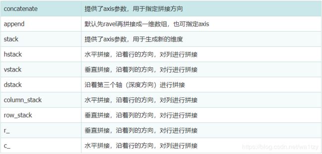
- 一、详解Numpy中的数组拼接、合并操作(concatenate, append, stack, hstack, vstack, r_, c_等)
- 二、Python字符串格式化
- 三、代码
前言
项目描述:根据鸢尾花的花萼长度与宽度的特征数据统计,对其进行逻辑回归分类。
特征:花萼长度、花萼宽度
类别标签:
0 - 山鸢尾(setosa)
1 - 杂色鸢尾(versicolor)
2 - 维吉尼亚鸢尾(virginica)
一、详解Numpy中的数组拼接、合并操作(concatenate, append, stack, hstack, vstack, r_, c_等)
二、Python字符串格式化

三、代码
思路:
(1)导入numpy,matplotlib,数据集
(2)加载数据
(3)取前100条样本和前两个特征
(4)分别取两类样本、数据分布可视化
(5)拆分样本,80个训练集(40个样本1,40个样本2),20个测试集(10个样本1,10个样本2)
(6)逻辑回归算法的实现
class logistic
def init
def sigmoid
def output
def compute_loss
def train
def predict
(7)创建实例,训练模型
# 导入numpy,matplotlib,数据集
import numpy as np
import matplotlib.pyplot as plt
from sklearn.datasets import load_iris

# iois 4个特征,3个类别,150个样本
# 加载数据
iris = load_iris()
# print(iris)
# print(iris.data)# 数据
# print(iris.target)# 标签
# print(iris.target_names)# 标签名
# print(iris.feature_names)# 特征名

# 取前100条样本和前两个特征
x = iris.data[0:100, 0:2]
y = iris.target[0:100]
# 分别取两类样本
samples_0 = x[y == 0, :]
samples_1 = x[y == 1, :]
# 数据分布可视化
plt.scatter(samples_0[:,0],samples_0[:,1],marker="o",c="r")
plt.scatter(samples_1[:,0],samples_1[:,1],marker="x",c="b")
plt.show()
# 拆分样本,80个训练集(训练,20个测试集(样本1有10个,样本2有10个)
x_train = np.vstack([x[:40], x[60:100]])
y_train = np.concatenate([y[:40], y[60:100]])
x_test = x[40:60, :]
y_test = y[40:60]

完整代码:
# 导入numpy,matplotlib,数据集
import numpy as np
import matplotlib.pyplot as plt
from sklearn.datasets import load_iris
class Logistic_Regression:
def __init__(self):
self.w = None
def sigmoid(self, z):
a = 1 / (1 + np.exp(-z))
return a
def output(self, x):
z = np.dot(self.w, x.T)
a = self.sigmoid(z)
return a
def compute_loss(self, x, y):
num_train = x.shape[0]# 样本数量
a = self.output(x)# 输出
loss = np.sum(-y * np.log(a) - (1 - y) * np.log(1 - a)) / num_train#所有样本的平均loss
dw = np.dot((a - y), x) / num_train# 平均梯度
return loss, dw
def train(self, x, y, lr=0.01, num_iterations=20000):
num_train, num_features = x.shape# 样本数、特征数(80,2)
self.w = 0.001 * np.random.randn(1, num_features)
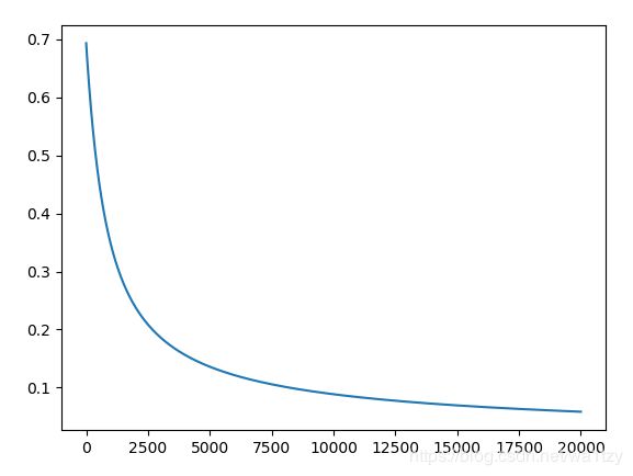
loss = []
for i in range(num_iterations):
error, dw = self.compute_loss(x, y)
loss.append(error)
self.w -= lr * dw
if i % 200 == 0:
print("step:[%d/%d],loss:%f" % (i, num_iterations, error))
return loss
def predict(self, x):
a = self.output(x)
y_pred = np.where(a >= 0.5, 1, 0)
return y_pred
iris = load_iris()
# 取前100条样本和前两个特征
x = iris.data[0:100, 0:2]
y = iris.target[0:100]
# 分别取两类样本
samples_0 = x[y == 0, :]
samples_1 = x[y == 1, :]
x_train = np.vstack([x[:40], x[60:100]])
y_train = np.concatenate([y[:40], y[60:100]])
x_test = x[40:60, :]
y_test = y[40:60]
lr = Logistic_Regression()
loss = lr.train(x_train, y_train)
# plt.plot(loss)
# plt.pause(0)
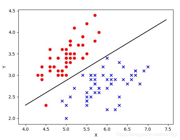
# 决策边界可视化
print(lr.w)# [[ 3.89311251 -6.76083755]]
"""
sigmoid = 1/(1+np.exp(-z))
x1*w1+x2*w2=0--> x2=-x1*w1/w2
"""
x1 = np.arange(4, 7.5, 0.05)
x2 = (-lr.w[0][0] * x1) / lr.w[0][1]
plt.scatter(samples_0[:, 0], samples_0[:, 1], marker="o", c="r")
plt.scatter(samples_1[:, 0], samples_1[:, 1], marker="x", c="b")
plt.xlabel("X")
plt.ylabel("Y")
plt.plot(x1, x2, "-", color="black")# 决策边界
plt.show()
num_test = x_test.shape[0]
prediction = lr.predict(x_test)
print(prediction)
print(y_test)
acc = np.sum(prediction == y_test)/num_test
print(acc)
out:
step:[0/20000],loss:0.693246
step:[200/20000],loss:0.577696
...
step:[19600/20000],loss:0.059064
step:[19800/20000],loss:0.058710
[[ 3.89314136 -6.760887  ]]
[[0 1 0 0 0 0 0 0 0 0 1 1 1 1 1 1 1 1 1 1]]
[0 0 0 0 0 0 0 0 0 0 1 1 1 1 1 1 1 1 1 1]
0.95