pandas项目之 房价预测项目:
项目:通过使用pandas对数据进行分析,采用Statsmodels 建立一元线性和多元线性回归模型
1、数据集说明
本项目用于分析的数据集主要右以下5个CSV文件:
- monthly-hpi.csv 文件:包含的信息
- date
- housing_price_index:房屋价格指数
- unemployment-macro.csv 文件:
- date
- total_unemployed:总失业人数
- more_than_15_week:超过15周都没有工作的人数
- not_in_labor_searched_for_work:没有再找工作
- multi_jobs:兼职多份工作
- leavers
- losers
- fed_funds.csv 文件:
- date
- federal_funds_rate:联邦基金利率
- shiller.csv 文件:
- date
- consumer_price_index :消费者物价指数
- long_interest_rate :长期的贷款利率
- gdp.csv:
- date
- gross_domestic_product :国内生产总值
- labor_force_pr : 人工价格
- product_price_index :商品的价格
2、 输入和输出的选择:
输出:房屋价格指数 housing_price_index
输入(就是自变量): 这个可以根据解决问题进行选择 。这个问题是基于房价预测的,因此我选择的因变量有:完全失业率total_unemployed实现一元线性回归。
3、使用pandas读取数据
首先:要将这五个文件都读取出来
federal_funds_rate = pd.read_csv(r"C:\Users\lab-635\Desktop\A3C\shixizhunbei\PD\price_of _house\fed_funds.csv")
gross_domestic_product = pd.read_csv(r"C:\Users\lab-635\Desktop\A3C\shixizhunbei\PD\price_of _house\gdp.csv")
house_price_index = pd.read_csv(r"C:\Users\lab-635\Desktop\A3C\shixizhunbei\PD\price_of _house\monthly-hpi.csv")
unemployment = pd.read_csv(r"C:\Users\lab-635\Desktop\A3C\shixizhunbei\PD\price_of _house\unemployment-macro.csv")
shiller = pd.read_csv(r"C:\Users\lab-635\Desktop\A3C\shixizhunbei\PD\price_of _house\shiller.csv")
在python中使用pandas 如果文件的列很多的话,不能直接显示出所有列的信息。需要在读取数据之前加入
pd.set_option('display.max_columns', None)通过head() 可以查看前五行的数据
print(federal_funds_rate.head())  # (贷款利率)
print(unemployment.head())   # 列:完全失业 / 超过15周的 /  /  多做几份工作的 / 自动辞职的 / 失败者
print(house_price_index.head())   # 时间和房价指数
print(gross_domestic_product.head()) # gdpv总共的消费 /  劳动价格  /商品的价格 / 国内生产总值
print(shiller.head())
4、利用pandas对数据进行整合
现在将所有数据合成一张总表格,按照date进行合并,因为这五张表格共有的列就是date列
df = shiller.merge(house_price_index,on = 'date')\
    .merge(unemployment, on = 'date')\
    .merge(federal_funds_rate,on = 'date')\
    .merge(gross_domestic_product,on = 'date')
5、简单的线性回归
简单的线性回归就是一个自变量来预测一个因变量,二者之间的关系可以用一条直线近似表示。
使用statemodels中的ols功能,构建房价和完全事业率之间的模型。OLS就是最小二乘法。
用法如下:
housing_model = ols(formula = 'housing_price_index ~ total_unemployed',data= df).fit()
housing_model_summary = housing_model.summary()
print(housing_model_summary)
输出的结果为:
OLS Regression Results
===============================================================================
Dep. Variable: housing_price_index R-squared: 0.952
Model: OLS Adj. R-squared: 0.949
Method: Least Squares F-statistic: 413.2
Date: Wed, 04 Mar 2020 Prob (F-statistic): 2.71e-15
Time: 18:56:42 Log-Likelihood: -65.450
No. Observations: 23 AIC: 134.9
Df Residuals: 21 BIC: 137.2
Df Model: 1
Covariance Type: nonrobust
====================================================================================
coef std err t P>|t| [0.025 0.975]
------------------------------------------------------------------------------------
Intercept 313.3128 5.408 57.938 0.000 302.067 324.559
total_unemployed -8.3324 0.410 -20.327 0.000 -9.185 -7.480
==============================================================================
Omnibus: 0.492 Durbin-Watson: 1.126
Prob(Omnibus): 0.782 Jarque-Bera (JB): 0.552
Skew: 0.294 Prob(JB): 0.759
Kurtosis: 2.521 Cond. No. 78.9
==============================================================================
主要数据分析:
Adj. R-squared: 0.949 。这个值表示 数据集中的94.9%的房屋价格指数与失业人数之间存在线性的关系
total_unemployed -8.3324 : 这个是回归洗漱,因变量前面的参数是 -8.3324
0.410 。 回归系数的标准误差。
6、线性回归图像
fig = plt.figure(figsize = (15,8))
fig = sm.graphics.plot_regress_exog(housing_model,'total_unemployed',fig = fig)  # '' 中的是取得名字
plt.show()
可以得到如下的图像:
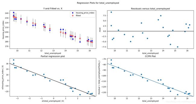
“Y and Fitted vs. X” :是房价观测值和线性估计值之间的差距。
“Residuals versus total_unemployed”:是上面图的放大版本。
Partial regression plot”:在考虑其他自变量的时候 房价和失业率的关系
“component and component-plus-residual(CCPR)”:
7、多元线性回归
考虑多个因变量 不仅仅只考虑失业人数,因此新增自变量:federal_funds_rate,long_interest_rate,consumer_price_index,gross_domestic_product。也采用最小二乘法。代码和之前的差不多,但是在因变量的部分需要进行改动
housing_model2 = ols(formula = """housing_price_index ~ total_unemployed
                              + long_interest_rate
                              +federal_funds_rate
                              + consumer_price_index
                            +gross_domestic_product """,data = df).fit()
housing_model2_summary = housing_model2.summary()
同时也会生成和之前差不多的表格:
OLS Regression Results
===============================================================================
Dep. Variable: housing_price_index R-squared: 0.980
Model: OLS Adj. R-squared: 0.974
Method: Least Squares F-statistic: 168.5
Date: Wed, 04 Mar 2020 Prob (F-statistic): 7.32e-14
Time: 19:17:31 Log-Likelihood: -55.164
No. Observations: 23 AIC: 122.3
Df Residuals: 17 BIC: 129.1
Df Model: 5
Covariance Type: nonrobust
==========================================================================================
coef std err t P>|t| [0.025 0.975]
------------------------------------------------------------------------------------------
Intercept -389.2234 187.252 -2.079 0.053 -784.291 5.844
total_unemployed -0.1727 2.399 -0.072 0.943 -5.234 4.889
long_interest_rate 5.4326 1.524 3.564 0.002 2.216 8.649
federal_funds_rate 32.3750 9.231 3.507 0.003 12.898 51.852
consumer_price_index 0.7785 0.360 2.164 0.045 0.020 1.537
gross_domestic_product 0.0252 0.010 2.472 0.024 0.004 0.047
==============================================================================
Omnibus: 1.363 Durbin-Watson: 1.899
Prob(Omnibus): 0.506 Jarque-Bera (JB): 1.043
Skew: -0.271 Prob(JB): 0.594
Kurtosis: 2.109 Cond. No. 4.58e+06
==============================================================================