- android系统selinux中添加新属性property
辉色投像
1.定位/android/system/sepolicy/private/property_contexts声明属性开头:persist.charge声明属性类型:u:object_r:system_prop:s0图12.定位到android/system/sepolicy/public/domain.te删除neverallow{domain-init}default_prop:property
- WPF中的ComboBox控件几种数据绑定的方式
互联网打工人no1
wpfc#
一、用字典给ItemsSource赋值(此绑定用的地方很多,建议熟练掌握)在XMAL中:在CS文件中privatevoidBindData(){DictionarydicItem=newDictionary();dicItem.add(1,"北京");dicItem.add(2,"上海");dicItem.add(3,"广州");cmb_list.ItemsSource=dicItem;cmb_l
- 将cmd中命令输出保存为txt文本文件
落难Coder
Windowscmdwindow
最近深度学习本地的训练中我们常常要在命令行中运行自己的代码,无可厚非,我们有必要保存我们的炼丹结果,但是复制命令行输出到txt是非常麻烦的,其实Windows下的命令行为我们提供了相应的操作。其基本的调用格式就是:运行指令>输出到的文件名称或者具体保存路径测试下,我打开cmd并且ping一下百度:pingwww.baidu.com>./data.txt看下相同目录下data.txt的输出:如果你再
- Linux MariaDB使用OpenSSL安装SSL证书
Meta39
MySQLOracleMariaDBLinuxWindowsssllinuxmariadb
进入到证书存放目录,批量删除.pem证书警告:确保已经进入到证书存放目录find.-typef-iname\*.pem-delete查看是否安装OpenSSLopensslversion没有则安装yuminstallopensslopenssl-devel开启SSL编辑/etc/my.cnf文件(没有的话就创建,但是要注意,在/etc/my.cnf.d/server.cnf配置了datadir的,
- 网络编程基础
记得开心一点啊
网络
目录♫什么是网络编程♫Socket套接字♪什么是Socket套接字♪数据报套接字♪流套接字♫数据报套接字通信模型♪数据报套接字通讯模型♪DatagramSocket♪DatagramPacket♪实现UDP的服务端代码♪实现UDP的客户端代码♫流套接字通信模型♪流套接字通讯模型♪ServerSocket♪Socket♪实现TCP的服务端代码♪实现TCP的客户端代码♫什么是网络编程网络编程,指网络上
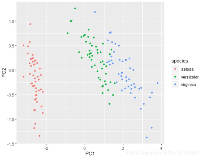
- K近邻算法_分类鸢尾花数据集
_feivirus_
算法机器学习和数学分类机器学习K近邻
importnumpyasnpimportpandasaspdfromsklearn.datasetsimportload_irisfromsklearn.model_selectionimporttrain_test_splitfromsklearn.metricsimportaccuracy_score1.数据预处理iris=load_iris()df=pd.DataFrame(data=ir
- 用Python实现读取统计单词个数
程序媛了了
python游戏java
完整实例代码:fromcollectionsimportCounterdefpythonit():danci={}withopen("pythonit.txt","r",encoding="utf-8")asf:foriinf:words=i.strip().split()forwordinwords:ifwordnotindanci:danci[word]=1else:danci[word]+=
- 4.C_数据结构_队列
荣世蓥
数据结构数据结构
概述什么是队列:队列是限定在两端进行插入操作和删除操作的线性表。具有先入先出(FIFO)的特点相关名词:队尾:写入数据的一段队头:读取数据的一段空队:队列中没有数据,队头指针=队尾指针满队:队列中存满了数据,队尾指针+1=队头指针循环队列1、基本内容循环队列是以数组形式构成的队列数据结构。循环队列的结构体如下:typedefintdata_t;//队列数据类型#defineN64//队列容量typ
- vue项目element-ui的table表格单元格合并
酋长哈哈
vue.jselementuijavascript前端
一、合并效果二全部代码exportdefault{name:'CellMerge',data(){return{tableData:[{id:'1',name:'王小虎',amount1:'165',amount2:'3.2',amount3:10},{id:'1',name:'王小虎',amount1:'162',amount2:'4.43',amount3:12},{id:'1',name:'
- python tif转png
Python与遥感
python开发语言
importosfromosgeoimportgdalimportnumpyasnpfromPILimportImage#提取432三波段fromspectralimport*#输入文件夹路径defget_img(dataset_img):width=dataset_img.RasterXSize#获取行列数height=dataset_img.RasterYSizebands=dataset_i
- MongoDB知识概括
GeorgeLin98
持久层mongodb
MongoDB知识概括MongoDB相关概念单机部署基本常用命令索引-IndexSpirngDataMongoDB集成副本集分片集群安全认证MongoDB相关概念业务应用场景:传统的关系型数据库(如MySQL),在数据操作的“三高”需求以及应对Web2.0的网站需求面前,显得力不从心。解释:“三高”需求:①Highperformance-对数据库高并发读写的需求。②HugeStorage-对海量数
- Vue中table合并单元格用法
weixin_30613343
javascriptViewUI
地名结果人名性别{{item.name}}已完成未完成{{item.groups[0].name}}{{item.groups[0].sex}}{{item.groups[son].name}}{{item.groups[son].sex}}exportdefault{data(){return{list:[{name:'地名1',result:'1',groups:[{name:'张三',sex
- 光盘文件系统 (iso9660) 格式解析
穷人小水滴
光盘文件系统iso9660denoGNU/Linuxjavascript
越简单的系统,越可靠,越不容易出问题.光盘文件系统(iso9660)十分简单,只需不到200行代码,即可实现定位读取其中的文件.参考资料:https://wiki.osdev.org/ISO_9660相关文章:《光盘防水嘛?DVD+R刻录光盘泡水实验》https://blog.csdn.net/secext2022/article/details/140583910《光驱的内部结构及日常使用》ht
- uniapp map组件自定义markers标记点
以对_
uni-app学习记录uni-appjavascript前端
需求是根据后端返回数据在地图上显示标记点,并且根据数据状态控制标记点颜色,标记点背景通过两张图片实现控制{{item.options.labelName}}exportdefault{data(){return{storeIndex:0,locaInfo:{longitude:120.445172,latitude:36.111387},markers:[//标点列表{id:1,//标记点idin
- 博客网站制作教程
2401_85194651
javamaven
首先就是技术框架:后端:Java+SpringBoot数据库:MySQL前端:Vue.js数据库连接:JPA(JavaPersistenceAPI)1.项目结构blog-app/├──backend/│├──src/main/java/com/example/blogapp/││├──BlogApplication.java││├──config/│││└──DatabaseConfig.java
- vue + Element UI table动态合并单元格
我家媳妇儿萌哒哒
elementUIvue.js前端javascript
一、功能需求1、根据名称相同的合并工作阶段和主要任务合并这两列,但主要任务内容一样,但要考虑主要任务一样,但工作阶段不一样的情况。(枞向合并)2、落实情况里的定量内容和定性内容值一样则合并。(横向合并)二、功能实现exportdefault{data(){return{tableData:[{name:'a',address:'1',age:'1',six:'2'},{name:'a',addre
- Python实现TIFF 文件转换为 PNG 和 JPG 格式
sand&wich
python开发语言
在日常的图像处理工作中,可能会遇到需要将TIFF格式的图像转换为其他格式的情况,例如PNG和JPG。下面,本文将介绍如何使用Python和GDAL库实现这一功能。准备工作在开始之前,请确保已经安装了必要的库:GDAL(GeospatialDataAbstractionLibrary)可以使用以下命令安装GDAL:pipinstallgdal代码实现以下是一个将TIFF文件转换为PNG文件的示例代码
- 《跃迁》5/7-5组-橙子-张静12.16
静言物于
【便签5】【片段来源】《跃迁:成为高手的技术》第四章【R原文】一位客户咨询时抱怨:“这个我做不到。”我问他:“如果我请你现在出去裸奔,你能做到吗?”“这个我也做不到”“其实并不是做不到,而是不愿意做,或者不想承担裸奔的代价吧。你不是做不到,而是选择不去做。如果有一天你裸奔能救自己家人、孩子,也许就能做到了。”为什么要做这个区分?如果一个人经常和自己说“做不到”,他的能力范围会越来越小,会成为一个无
- ✔2848. 与车相交的点
程序员小小聪
力扣leetcode
代码实现:方法一:哈希表#definefmax(a,b)((a)>(b)?(a):(b))intnumberOfPoints(int**nums,intnumsSize,int*numsColSize){inthash[101]={0};intmax=0;for(inti=0;i=x){j--;}if(i=nums[i][0]){r=r>nums[i][1]?r:nums[i][1];}else{
- 【加密算法基础——RSA 加密】
XWWW668899
网络服务器笔记python
RSA加密RSA(Rivest-Shamir-Adleman)加密是非对称加密,一种广泛使用的公钥加密算法,主要用于安全数据传输。公钥用于加密,私钥用于解密。RSA加密算法的名称来源于其三位发明者的姓氏:R:RonRivestS:AdiShamirA:LeonardAdleman这三位计算机科学家在1977年共同提出了这一算法,并发表了相关论文。他们的工作为公钥加密的基础奠定了重要基础,使得安全通
- 使用datepicker和uploadify的冲突解决(IE双击才能打开附件上传对话框)
zhanglb12
在开发的过程当中,IE的兼容无疑是我们的一块绊脚石,在我们使用的如期的datepicker插件和使用上传附件的uploadify插件的时候,两者就产生冲突,只要点击过时间的插件,uploadify上传框要双才能打开ie浏览器提示错误Missinginstancedataforthisdatepicker解决方案//if(.browser.msie&&'9.0'===.browser.version
- golang获取用户输入的几种方式
余生逆风飞翔
golang开发语言后端
一、定义结构体typeUserInfostruct{Namestring`json:"name"`Ageint`json:"age"`Addstring`json:"add"`}typeReturnDatastruct{Messagestring`json:"message"`Statusstring`json:"status"`DataUserInfo`json:"data"`}二、get请求的
- 【Java】已解决:org.springframework.jdbc.datasource.lookup.DataSourceLookupFailureException
屿小夏
java开发语言
文章目录一、分析问题背景问题背景描述出现问题的场景二、可能出错的原因三、错误代码示例四、正确代码示例五、注意事项已解决:org.springframework.jdbc.datasource.lookup.DataSourceLookupFailureException在使用Spring框架进行开发时,数据源的配置和使用是非常关键的一环。然而,有时候我们可能会遇到org.springframewo
- el-table实现全选整表,单元一页复选框功能
周bro
vue.jselementuijavascript前端
全选整表单选一页0":popper-append-to-body="false":total="tableData.length":page-size="pageObj.pagesize":page-sizes="[10,50,100]"layout="total,sizes,prev,pager,next"@size-change="handleSizeChange"@current-chang
- Acwing 区间合并
Curry_Math
算法学习算法c++开发语言
区间合并主要思想:给定很多区间。若两个区间有交集,将二者合并成一个区间。具体做法:先按照区间的左端点进行排序然后遍历每个区间,根据不同的情况进行合并,有一下几种情况:第一种情况,区间不变;第二种情况,end更新为区间i的右端点;以上两种情况,可以归结为end更新为max(end,r);r为区间右端点第三种情况,将当前维护的区间加入结果,并将维护的区间更新为区间i;下面给出区间合并的板子://区间合
- Android shell 常用 debug 命令
晨春计
Audiodebugandroidlinux
目录1、查看版本2、am命令3、pm命令4、dumpsys命令5、sed命令6、log定位查看APK进程号7、log定位使用场景1、查看版本1.1、Android串口终端执行getpropro.build.version.release#获取Android版本uname-a#查看linux内核版本信息uname-r#单独查看内核版本1.2、linux服务器执行lsb_release-a#查看Lin
- Vue + Express实现一个表单提交
九旬大爷的梦
最近在折腾一个cms系统,用的vue+express,但是就一个表单提交就弄了好久,记录一下。环境:Node10+前端:Vue服务端:Express依赖包:vueexpressaxiosexpress-formidableelement-ui(可选)前言:axiosget请求参数是:paramsaxiospost请求参数是:dataexpressget接受参数是req.queryexpresspo
- 大牛:新型电动汽车电池技术问世! 可将电池能量密度提高2倍成本降一半
38cc8b780dc0
据外媒报道,当地时间6月10日,电动汽车电池技术领导者OneDBatterySciences宣布推出一项可为下一代电动汽车电池提供动力的突破性技术——SINANODE。对于电动汽车行业而言,打造含有更多硅的电池一直是一个挑战,而SINANODE无缝集成至现有的生产工艺中,让硅纳米线与商用石墨粉末融合,将电池阳极的能量密度提高了两倍,但是将每kWh的成本降低了一半。能量密度更高可以让电池的续航更长,
- Kubernetes部署MySQL数据持久化
沫殇-MS
KubernetesMySQL数据库kubernetesmysql容器
一、安装配置NFS服务端1、安装nfs-kernel-server:sudoapt-yinstallnfs-kernel-server2、服务端创建共享目录#列出所有可用块设备的信息lsblk#格式化磁盘sudomkfs-text4/dev/sdb#创建一个目录:sudomkdir-p/data/nfs/mysql#更改目录权限:sudochown-Rnobody:nogroup/data/nfs
- Hadoop架构
henan程序媛
hadoop大数据分布式
一、案列分析1.1案例概述现在已经进入了大数据(BigData)时代,数以万计用户的互联网服务时时刻刻都在产生大量的交互,要处理的数据量实在是太大了,以传统的数据库技术等其他手段根本无法应对数据处理的实时性、有效性的需求。HDFS顺应时代出现,在解决大数据存储和计算方面有很多的优势。1.2案列前置知识点1.什么是大数据大数据是指无法在一定时间范围内用常规软件工具进行捕捉、管理和处理的大量数据集合,
- Java开发中,spring mvc 的线程怎么调用?
小麦麦子
springmvc
今天逛知乎,看到最近很多人都在问spring mvc 的线程http://www.maiziedu.com/course/java/ 的启动问题,觉得挺有意思的,那哥们儿问的也听仔细,下面的回答也很详尽,分享出来,希望遇对遇到类似问题的Java开发程序猿有所帮助。
问题:
在用spring mvc架构的网站上,设一线程在虚拟机启动时运行,线程里有一全局
- maven依赖范围
bitcarter
maven
1.test 测试的时候才会依赖,编译和打包不依赖,如junit不被打包
2.compile 只有编译和打包时才会依赖
3.provided 编译和测试的时候依赖,打包不依赖,如:tomcat的一些公用jar包
4.runtime 运行时依赖,编译不依赖
5.默认compile
依赖范围compile是支持传递的,test不支持传递
1.传递的意思是项目A,引用
- Jaxb org.xml.sax.saxparseexception : premature end of file
darrenzhu
xmlprematureJAXB
如果在使用JAXB把xml文件unmarshal成vo(XSD自动生成的vo)时碰到如下错误:
org.xml.sax.saxparseexception : premature end of file
很有可能时你直接读取文件为inputstream,然后将inputstream作为构建unmarshal需要的source参数。InputSource inputSource = new In
- CSS Specificity
周凡杨
html权重Specificitycss
有时候对于页面元素设置了样式,可为什么页面的显示没有匹配上呢? because specificity
CSS 的选择符是有权重的,当不同的选择符的样式设置有冲突时,浏览器会采用权重高的选择符设置的样式。
规则:
HTML标签的权重是1
Class 的权重是10
Id 的权重是100
- java与servlet
g21121
servlet
servlet 搞java web开发的人一定不会陌生,而且大家还会时常用到它。
下面是java官方网站上对servlet的介绍: java官网对于servlet的解释 写道
Java Servlet Technology Overview Servlets are the Java platform technology of choice for extending and enha
- eclipse中安装maven插件
510888780
eclipsemaven
1.首先去官网下载 Maven:
http://www.apache.org/dyn/closer.cgi/maven/binaries/apache-maven-3.2.3-bin.tar.gz
下载完成之后将其解压,
我将解压后的文件夹:apache-maven-3.2.3,
并将它放在 D:\tools目录下,
即 maven 最终的路径是:D:\tools\apache-mave
- jpa@OneToOne关联关系
布衣凌宇
jpa
Nruser里的pruserid关联到Pruser的主键id,实现对一个表的增删改,另一个表的数据随之增删改。
Nruser实体类
//*****************************************************************
@Entity
@Table(name="nruser")
@DynamicInsert @Dynam
- 我的spring学习笔记11-Spring中关于声明式事务的配置
aijuans
spring事务配置
这两天学到事务管理这一块,结合到之前的terasoluna框架,觉得书本上讲的还是简单阿。我就把我从书本上学到的再结合实际的项目以及网上看到的一些内容,对声明式事务管理做个整理吧。我看得Spring in Action第二版中只提到了用TransactionProxyFactoryBean和<tx:advice/>,定义注释驱动这三种,我承认后两种的内容很好,很强大。但是实际的项目当中
- java 动态代理简单实现
antlove
javahandlerproxydynamicservice
dynamicproxy.service.HelloService
package dynamicproxy.service;
public interface HelloService {
public void sayHello();
}
dynamicproxy.service.impl.HelloServiceImpl
package dynamicp
- JDBC连接数据库
百合不是茶
JDBC编程JAVA操作oracle数据库
如果我们要想连接oracle公司的数据库,就要首先下载oralce公司的驱动程序,将这个驱动程序的jar包导入到我们工程中;
JDBC链接数据库的代码和固定写法;
1,加载oracle数据库的驱动;
&nb
- 单例模式中的多线程分析
bijian1013
javathread多线程java多线程
谈到单例模式,我们立马会想到饿汉式和懒汉式加载,所谓饿汉式就是在创建类时就创建好了实例,懒汉式在获取实例时才去创建实例,即延迟加载。
饿汉式:
package com.bijian.study;
public class Singleton {
private Singleton() {
}
// 注意这是private 只供内部调用
private static
- javascript读取和修改原型特别需要注意原型的读写不具有对等性
bijian1013
JavaScriptprototype
对于从原型对象继承而来的成员,其读和写具有内在的不对等性。比如有一个对象A,假设它的原型对象是B,B的原型对象是null。如果我们需要读取A对象的name属性值,那么JS会优先在A中查找,如果找到了name属性那么就返回;如果A中没有name属性,那么就到原型B中查找name,如果找到了就返回;如果原型B中也没有
- 【持久化框架MyBatis3六】MyBatis3集成第三方DataSource
bit1129
dataSource
MyBatis内置了数据源的支持,如:
<environments default="development">
<environment id="development">
<transactionManager type="JDBC" />
<data
- 我程序中用到的urldecode和base64decode,MD5
bitcarter
cMD5base64decodeurldecode
这里是base64decode和urldecode,Md5在附件中。因为我是在后台所以需要解码:
string Base64Decode(const char* Data,int DataByte,int& OutByte)
{
//解码表
const char DecodeTable[] =
{
0, 0, 0, 0, 0, 0
- 腾讯资深运维专家周小军:QQ与微信架构的惊天秘密
ronin47
社交领域一直是互联网创业的大热门,从PC到移动端,从OICQ、MSN到QQ。到了移动互联网时代,社交领域应用开始彻底爆发,直奔黄金期。腾讯在过去几年里,社交平台更是火到爆,QQ和微信坐拥几亿的粉丝,QQ空间和朋友圈各种刷屏,写心得,晒照片,秀视频,那么谁来为企鹅保驾护航呢?支撑QQ和微信海量数据背后的架构又有哪些惊天内幕呢?本期大讲堂的内容来自今年2月份ChinaUnix对腾讯社交网络运营服务中心
- java-69-旋转数组的最小元素。把一个数组最开始的若干个元素搬到数组的末尾,我们称之为数组的旋转。输入一个排好序的数组的一个旋转,输出旋转数组的最小元素
bylijinnan
java
public class MinOfShiftedArray {
/**
* Q69 旋转数组的最小元素
* 把一个数组最开始的若干个元素搬到数组的末尾,我们称之为数组的旋转。输入一个排好序的数组的一个旋转,输出旋转数组的最小元素。
* 例如数组{3, 4, 5, 1, 2}为{1, 2, 3, 4, 5}的一个旋转,该数组的最小值为1。
*/
publ
- 看博客,应该是有方向的
Cb123456
反省看博客
看博客,应该是有方向的:
我现在就复习以前的,在补补以前不会的,现在还不会的,同时完善完善项目,也看看别人的博客.
我刚突然想到的:
1.应该看计算机组成原理,数据结构,一些算法,还有关于android,java的。
2.对于我,也快大四了,看一些职业规划的,以及一些学习的经验,看看别人的工作总结的.
为什么要写
- [开源与商业]做开源项目的人生活上一定要朴素,尽量减少对官方和商业体系的依赖
comsci
开源项目
为什么这样说呢? 因为科学和技术的发展有时候需要一个平缓和长期的积累过程,但是行政和商业体系本身充满各种不稳定性和不确定性,如果你希望长期从事某个科研项目,但是却又必须依赖于某种行政和商业体系,那其中的过程必定充满各种风险。。。
所以,为避免这种不确定性风险,我
- 一个 sql优化 ([精华] 一个查询优化的分析调整全过程!很值得一看 )
cwqcwqmax9
sql
见 http://www.itpub.net/forum.php?mod=viewthread&tid=239011
Web翻页优化实例
提交时间: 2004-6-18 15:37:49 回复 发消息
环境:
Linux ve
- Hibernat and Ibatis
dashuaifu
Hibernateibatis
Hibernate VS iBATIS 简介 Hibernate 是当前最流行的O/R mapping框架,当前版本是3.05。它出身于sf.net,现在已经成为Jboss的一部分了 iBATIS 是另外一种优秀的O/R mapping框架,当前版本是2.0。目前属于apache的一个子项目了。 相对Hibernate“O/R”而言,iBATIS 是一种“Sql Mappi
- 备份MYSQL脚本
dcj3sjt126com
mysql
#!/bin/sh
# this shell to backup mysql
#
[email protected] (QQ:1413161683 DuChengJiu)
_dbDir=/var/lib/mysql/
_today=`date +%w`
_bakDir=/usr/backup/$_today
[ ! -d $_bakDir ] && mkdir -p
- iOS第三方开源库的吐槽和备忘
dcj3sjt126com
ios
转自
ibireme的博客 做iOS开发总会接触到一些第三方库,这里整理一下,做一些吐槽。 目前比较活跃的社区仍旧是Github,除此以外也有一些不错的库散落在Google Code、SourceForge等地方。由于Github社区太过主流,这里主要介绍一下Github里面流行的iOS库。 首先整理了一份
Github上排名靠
- html wlwmanifest.xml
eoems
htmlxml
所谓优化wp_head()就是把从wp_head中移除不需要元素,同时也可以加快速度。
步骤:
加入到function.php
remove_action('wp_head', 'wp_generator');
//wp-generator移除wordpress的版本号,本身blog的版本号没什么意义,但是如果让恶意玩家看到,可能会用官网公布的漏洞攻击blog
remov
- 浅谈Java定时器发展
hacksin
java并发timer定时器
java在jdk1.3中推出了定时器类Timer,而后在jdk1.5后由Dou Lea从新开发出了支持多线程的ScheduleThreadPoolExecutor,从后者的表现来看,可以考虑完全替代Timer了。
Timer与ScheduleThreadPoolExecutor对比:
1.
Timer始于jdk1.3,其原理是利用一个TimerTask数组当作队列
- 移动端页面侧边导航滑入效果
ini
jqueryWebhtml5cssjavascirpt
效果体验:http://hovertree.com/texiao/mobile/2.htm可以使用移动设备浏览器查看效果。效果使用到jquery-2.1.4.min.js,该版本的jQuery库是用于支持HTML5的浏览器上,不再兼容IE8以前的浏览器,现在移动端浏览器一般都支持HTML5,所以使用该jQuery没问题。HTML文件代码:
<!DOCTYPE html>
<h
- AspectJ+Javasist记录日志
kane_xie
aspectjjavasist
在项目中碰到这样一个需求,对一个服务类的每一个方法,在方法开始和结束的时候分别记录一条日志,内容包括方法名,参数名+参数值以及方法执行的时间。
@Override
public String get(String key) {
// long start = System.currentTimeMillis();
// System.out.println("Be
- redis学习笔记
MJC410621
redisNoSQL
1)nosql数据库主要由以下特点:非关系型的、分布式的、开源的、水平可扩展的。
1,处理超大量的数据
2,运行在便宜的PC服务器集群上,
3,击碎了性能瓶颈。
1)对数据高并发读写。
2)对海量数据的高效率存储和访问。
3)对数据的高扩展性和高可用性。
redis支持的类型:
Sring 类型
set name lijie
get name lijie
set na
- 使用redis实现分布式锁
qifeifei
在多节点的系统中,如何实现分布式锁机制,其中用redis来实现是很好的方法之一,我们先来看一下jedis包中,有个类名BinaryJedis,它有个方法如下:
public Long setnx(final byte[] key, final byte[] value) {
checkIsInMulti();
client.setnx(key, value);
ret
- BI并非万能,中层业务管理报表要另辟蹊径
张老师的菜
大数据BI商业智能信息化
BI是商业智能的缩写,是可以帮助企业做出明智的业务经营决策的工具,其数据来源于各个业务系统,如ERP、CRM、SCM、进销存、HER、OA等。
BI系统不同于传统的管理信息系统,他号称是一个整体应用的解决方案,是融入管理思想的强大系统:有着系统整体的设计思想,支持对所有
- 安装rvm后出现rvm not a function 或者ruby -v后提示没安装ruby的问题
wudixiaotie
function
1.在~/.bashrc最后加入
[[ -s "$HOME/.rvm/scripts/rvm" ]] && source "$HOME/.rvm/scripts/rvm"
2.重新启动terminal输入:
rvm use ruby-2.2.1 --default
把当前安装的ruby版本设为默