优衣库销售数据分析

#1.加载工具包
import pandas as pd
import matplotlib.pyplot as plt
import seaborn as sns
%matplotlib inline

#加载优衣库文件
UNIQLO=pd.read_csv('L2W1.csv')
#清理数据，描述性语句查看缺失值，去掉销售额为负数的结果
UNIQLO.head()

	store_id	city	channel	gender_group	age_group	wkd_ind	product	customer	revenue	order	quant	unit_cost
0	658	深圳	线下	Female	25-29	Weekday	当季新品	4	796.0	4	4	59
1	146	杭州	线下	Female	25-29	Weekday	运动	1	149.0	1	1	49
2	70	深圳	线下	Male	>=60	Weekday	T恤	2	178.0	2	2	49
3	658	深圳	线下	Female	25-29	Weekday	T恤	1	59.0	1	1	49
4	229	深圳	线下	Male	20-24	Weekend	袜子	2	65.0	2	3	9

UNIQLO.info()#无缺失值
UNIQLO.describe()

RangeIndex: 22293 entries, 0 to 22292
Data columns (total 12 columns):
store_id        22293 non-null int64
city            22293 non-null object
channel         22293 non-null object
gender_group    22293 non-null object
age_group       22293 non-null object
wkd_ind         22293 non-null object
product         22293 non-null object
customer        22293 non-null int64
revenue         22293 non-null float64
order           22293 non-null int64
quant           22293 non-null int64
unit_cost       22293 non-null int64
dtypes: float64(1), int64(5), object(6)
memory usage: 2.0+ MB

	store_id	customer	revenue	order	quant	unit_cost
count	22293.000000	22293.000000	22293.000000	22293.000000	22293.000000	22293.000000
mean	335.391558	1.629480	159.531371	1.651998	1.858072	46.124658
std	230.236167	1.785605	276.254066	1.861480	2.347301	19.124347
min	19.000000	1.000000	-0.660000	1.000000	1.000000	9.000000
25%	142.000000	1.000000	64.000000	1.000000	1.000000	49.000000
50%	315.000000	1.000000	99.000000	1.000000	1.000000	49.000000
75%	480.000000	2.000000	175.000000	2.000000	2.000000	49.000000
max	831.000000	58.000000	12538.000000	65.000000	84.000000	99.000000

UNIQLO1 = UNIQLO[UNIQLO['revenue']>0]
UNIQLO1.describe()

	store_id	customer	revenue	order	quant	unit_cost
count	22262.000000	22262.000000	22262.000000	22262.000000	22262.000000	22262.000000
mean	335.486614	1.630357	159.753549	1.652906	1.859222	46.127841
std	230.371454	1.786694	276.382135	1.862617	2.348723	19.120825
min	19.000000	1.000000	10.000000	1.000000	1.000000	9.000000
25%	142.000000	1.000000	66.000000	1.000000	1.000000	49.000000
50%	315.000000	1.000000	99.000000	1.000000	1.000000	49.000000
75%	480.000000	2.000000	175.000000	2.000000	2.000000	49.000000
max	831.000000	58.000000	12538.000000	65.000000	84.000000	99.000000

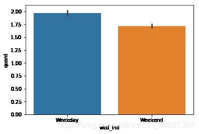
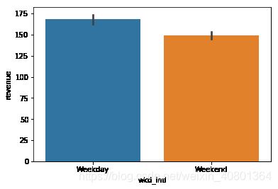
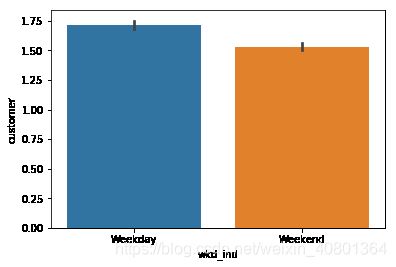
问题一：整体销售情况随着时间的变化是怎样的？

题目拆解：
数据中与时间有关的字段仅为类别变量wkd_ind代表的Weekday和Weekend，即购买发生的时间是周中还是周末。本题意为分析对比周末和周中与销售有关的数据，包括产品销售数量quant、销售金额revenue、顾客人数customer的情况，可生成柱状图进行可视化。

sns.barplot(x='wkd_ind',y='quant',data =UNIQLO1)

C:\Users\LYY\Anaconda3\lib\site-packages\scipy\stats\stats.py:1713: FutureWarning: Using a non-tuple sequence for multidimensional indexing is deprecated; use `arr[tuple(seq)]` instead of `arr[seq]`. In the future this will be interpreted as an array index, `arr[np.array(seq)]`, which will result either in an error or a different result.
  return np.add.reduce(sorted[indexer] * weights, axis=axis) / sumval

sns.barplot(x='wkd_ind',y='revenue',data =UNIQLO1)

C:\Users\LYY\Anaconda3\lib\site-packages\scipy\stats\stats.py:1713: FutureWarning: Using a non-tuple sequence for multidimensional indexing is deprecated; use `arr[tuple(seq)]` instead of `arr[seq]`. In the future this will be interpreted as an array index, `arr[np.array(seq)]`, which will result either in an error or a different result.
  return np.add.reduce(sorted[indexer] * weights, axis=axis) / sumval

sns.barplot(x='wkd_ind',y='customer',data =UNIQLO1)

C:\Users\LYY\Anaconda3\lib\site-packages\scipy\stats\stats.py:1713: FutureWarning: Using a non-tuple sequence for multidimensional indexing is deprecated; use `arr[tuple(seq)]` instead of `arr[seq]`. In the future this will be interpreted as an array index, `arr[np.array(seq)]`, which will result either in an error or a different result.
  return np.add.reduce(sorted[indexer] * weights, axis=axis) / sumval

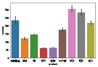
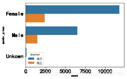
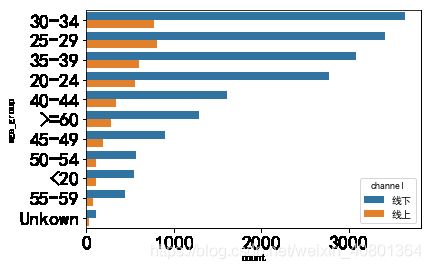
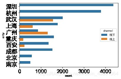
问题二：不同产品的销售情况是怎样的？顾客偏爱哪一种购买方式？

题目拆解：

• 不同产品即指product字段中不同类别的产品，销售情况即为销售额revenue，可生成柱状图进行可视化
• 购买方式只有channel是线上还是线下这一个指标，而顾客可以从不同性别gender_group、年龄段age_group、城市city三个维度进行分解，因此本问即为探究不同性别、年龄段和城市的顾客对线上、线下两种购买方式的偏好，可生成柱状图进行可视化的呈现

UNIQLO1.groupby(['product'])['revenue'].describe()

	count	mean	std	min	25%	50%	75%	max
product
T恤	10598.0	145.192002	154.288788	13.50	79.0	99.0	158.0	6636.00
当季新品	2534.0	233.095848	597.852857	19.00	76.0	111.0	197.0	12538.00
毛衣	806.0	304.752854	290.715612	13.00	149.0	199.0	396.0	4975.00
牛仔裤	1410.0	174.558496	238.760626	13.33	59.0	79.0	199.0	2087.00
短裤	1691.0	63.563501	55.631526	10.00	37.0	40.0	77.0	676.00
袜子	2048.0	62.368828	51.153136	10.00	27.0	52.0	79.0	595.36
裙子	629.0	218.287409	172.449212	10.00	99.0	197.0	237.0	1442.00
运动	975.0	121.087528	142.760425	18.00	39.0	78.0	149.0	1257.00
配件	1571.0	283.058657	398.768068	29.00	99.0	149.0	298.0	4187.00

#u_plot = UNIQLO1.groupby(['product'])['revenue']
#解决中文和负号不正常显示问题
plt.rcParams['font.sans-serif'] = 'SimHei'
plt.rcParams['axes.unicode_minus'] = False
sns.barplot(x = 'product',y = 'revenue',data = UNIQLO1)
#这个地方怎么排序

C:\Users\LYY\Anaconda3\lib\site-packages\scipy\stats\stats.py:1713: FutureWarning: Using a non-tuple sequence for multidimensional indexing is deprecated; use `arr[tuple(seq)]` instead of `arr[seq]`. In the future this will be interpreted as an array index, `arr[np.array(seq)]`, which will result either in an error or a different result.
  return np.add.reduce(sorted[indexer] * weights, axis=axis) / sumval

1.从不同性别gender_group

plt.rcParams['font.sans-serif'] = 'SimHei'
plt.rcParams['axes.unicode_minus'] = False
sns.countplot(y='gender_group',hue='channel',data=UNIQLO1,order=UNIQLO1['gender_group'].value_counts().index)
plt.tick_params(labelsize=20)

plt.rcParams['font.sans-serif'] = 'SimHei'
plt.rcParams['axes.unicode_minus'] = False
sns.countplot(y='age_group',hue='channel',data=UNIQLO1,order=UNIQLO1['age_group'].value_counts().index)
plt.tick_params(labelsize=20)

plt.rcParams['font.sans-serif'] = 'SimHei'
plt.rcParams['axes.unicode_minus'] = False
sns.countplot(y='city',hue='channel',data=UNIQLO1,order=UNIQLO1['city'].value_counts().index)
plt.tick_params(labelsize=20)

问题三：销售额和产品成本之间的关系怎么样？

题目拆解：

• 每单顾客的总销售额为revenue，根据数量quant可以计算出单件产品销售金额，又已知单件产品成本为unit_cost和其类别product。
• 思路一：单件产品销售额-成本为利润margin，margin是如何分布的？是否存在亏本销售的产品？
• 思路二：探究实际销售额和产品成本之间的关系，即为求它们之间的相关，若成正相关，则产品成本越高，销售额越高，或许为高端商品；若成负相关，则成本越低，销售额越高，为薄利多销的模式。

• 还可以拆分得更细，探究不同城市和门店中成本和销售额的相关性。

UNIQLO1.head()

	store_id	city	channel	gender_group	age_group	wkd_ind	product	customer	revenue	order	quant	unit_cost
0	658	深圳	线下	Female	25-29	Weekday	当季新品	4	796.0	4	4	59
1	146	杭州	线下	Female	25-29	Weekday	运动	1	149.0	1	1	49
2	70	深圳	线下	Male	>=60	Weekday	T恤	2	178.0	2	2	49
3	658	深圳	线下	Female	25-29	Weekday	T恤	1	59.0	1	1	49
4	229	深圳	线下	Male	20-24	Weekend	袜子	2	65.0	2	3	9

UNIQLO1['unit_revenue'] = (UNIQLO1['revenue']/UNIQLO1['quant'])
UNIQLO1['margin'] = (UNIQLO1['revenue']/UNIQLO1['quant']-UNIQLO1['unit_cost'])

C:\Users\LYY\Anaconda3\lib\site-packages\ipykernel_launcher.py:1: SettingWithCopyWarning: 
A value is trying to be set on a copy of a slice from a DataFrame.
Try using .loc[row_indexer,col_indexer] = value instead

See the caveats in the documentation: http://pandas.pydata.org/pandas-docs/stable/indexing.html#indexing-view-versus-copy
  """Entry point for launching an IPython kernel.
C:\Users\LYY\Anaconda3\lib\site-packages\ipykernel_launcher.py:2: SettingWithCopyWarning: 
A value is trying to be set on a copy of a slice from a DataFrame.
Try using .loc[row_indexer,col_indexer] = value instead

See the caveats in the documentation: http://pandas.pydata.org/pandas-docs/stable/indexing.html#indexing-view-versus-copy

UNIQLO1.head()

	store_id	city	channel	gender_group	age_group	wkd_ind	product	customer	revenue	order	quant	unit_cost	unit_revenue	profit	margin
0	658	深圳	线下	Female	25-29	Weekday	当季新品	4	796.0	4	4	59	199.000000	140.000000	140.000000
1	146	杭州	线下	Female	25-29	Weekday	运动	1	149.0	1	1	49	149.000000	100.000000	100.000000
2	70	深圳	线下	Male	>=60	Weekday	T恤	2	178.0	2	2	49	89.000000	40.000000	40.000000
3	658	深圳	线下	Female	25-29	Weekday	T恤	1	59.0	1	1	49	59.000000	10.000000	10.000000
4	229	深圳	线下	Male	20-24	Weekend	袜子	2	65.0	2	3	9	21.666667	12.666667	12.666667

#单件产品的利润的分布，存在收入为负的情况
sns.distplot(UNIQLO1['margin'])

C:\Users\LYY\Anaconda3\lib\site-packages\scipy\stats\stats.py:1713: FutureWarning: Using a non-tuple sequence for multidimensional indexing is deprecated; use `arr[tuple(seq)]` instead of `arr[seq]`. In the future this will be interpreted as an array index, `arr[np.array(seq)]`, which will result either in an error or a different result.
  return np.add.reduce(sorted[indexer] * weights, axis=axis) / sumval

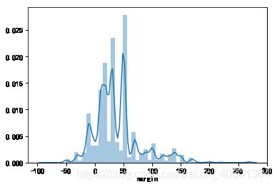
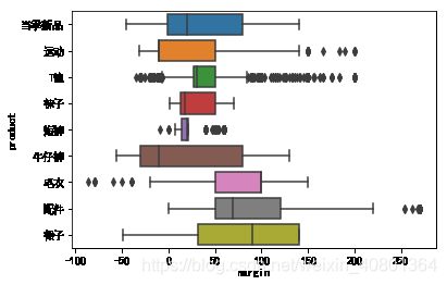
销售产品的利润分布(类别)

• 牛仔裤最可能成为亏本销售产品，部分的毛衣和T恤也可能存在亏本销售；
• T恤的盈利的波动较大，-50到200
• 裙子和配件是盈利比较高的两类商品

sns.boxplot(x='margin',y = 'product',data = UNIQLO1)

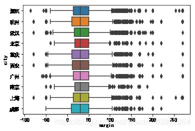
销售产品的利润分布（城市）

• 各城市表现类似

sns.boxplot(x='margin',y = 'city',data = UNIQLO1)

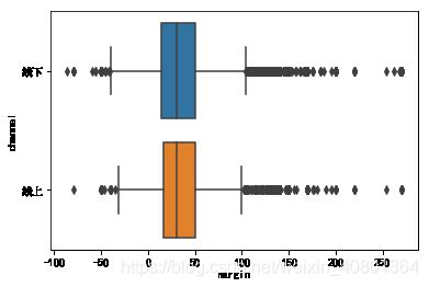
sns.boxplot(x='margin',y = 'channel',data = UNIQLO1)

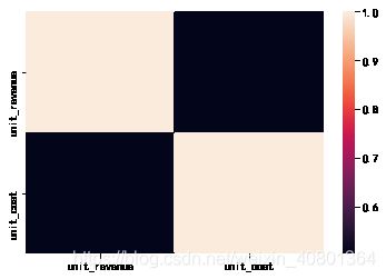
#探究实际销售额和产品成本之间的关系,R值为0.5，成本越高，销售额越高，可能是高端商品占主要？？
UNIQLO1[['unit_revenue','unit_cost']].corr()

	unit_revenue	unit_cost
unit_revenue	1.000000	0.503499
unit_cost	0.503499	1.000000

sns.heatmap(UNIQLO1[['unit_revenue','unit_cost']].corr())

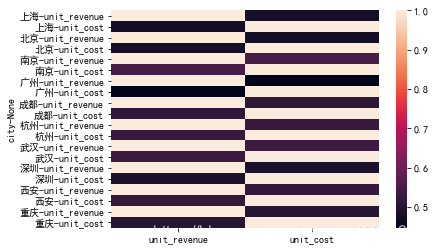
还可以拆分得更细，探究不同城市和门店中成本和销售额的相关性

UNIQLO1.groupby(['city'])['unit_revenue','unit_cost'].corr(min_periods=1)

		unit_revenue	unit_cost
city
上海	unit_revenue	1.000000	0.475711
	unit_cost	0.475711	1.000000
北京	unit_revenue	1.000000	0.474852
	unit_cost	0.474852	1.000000
南京	unit_revenue	1.000000	0.550571
	unit_cost	0.550571	1.000000
广州	unit_revenue	1.000000	0.446615
	unit_cost	0.446615	1.000000
成都	unit_revenue	1.000000	0.514083
	unit_cost	0.514083	1.000000
杭州	unit_revenue	1.000000	0.529296
	unit_cost	0.529296	1.000000
武汉	unit_revenue	1.000000	0.536779
	unit_cost	0.536779	1.000000
深圳	unit_revenue	1.000000	0.487396
	unit_cost	0.487396	1.000000
西安	unit_revenue	1.000000	0.523069
	unit_cost	0.523069	1.000000
重庆	unit_revenue	1.000000	0.504232
	unit_cost	0.504232	1.000000

sns.heatmap(UNIQLO1.groupby(['city'])['unit_revenue','unit_cost'].corr())

不同城市成本和销售额的相关性比较一致，其中南京相关性稍微强一些