sklearn 实现简单回归算法
线性回归和逻辑回归,基本概念可以去参照前一篇文章。这一篇主要以例题形式。代码解释与实现。
1.
from sklearn import datasets   #sklearn自带数据集,实战使用时数据用read。。。导入
from sklearn.model_selection import cross_val_predict  #做交叉验证预测的函数导入
from sklearn import linear_model   #线性规划
import matplotlib.pyplot as plt  #可视化库

lr = linear_model.LinearRegression()   #线性回归算法
boston = datasets.load_boston()        #导入数据集
y = boston.target
print(boston)

# cross_val_predict returns an array of the same size as `y` where each entry
# is a prediction obtained by cross validation:
predicted = cross_val_predict(lr, boston.data, y, cv=10)#交叉预测
# lr.fit(x)    #不用交叉验证预测时的训练模型
#  lr.predict(y)#预测结果
fig, ax = plt.subplots()
ax.scatter(y, predicted, edgecolors=(0, 0, 0))
ax.plot([y.min(), y.max()], [y.min(), y.max()], 'k--', lw=4)
ax.set_xlabel('Measured')
ax.set_ylabel('Predicted')
plt.show()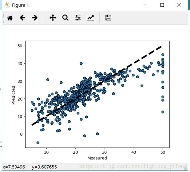
2.Isotonic Regression
import numpy as np
import matplotlib.pyplot as plt
from matplotlib.collections import LineCollection

from sklearn.linear_model import LinearRegression
from sklearn.isotonic import IsotonicRegression
from sklearn.utils import check_random_state

n = 100
x = np.arange(n)
rs = check_random_state(0)
y = rs.randint(-50, 50, size=(n,)) + 50. * np.log(1 + np.arange(n))

# #############################################################################
# Fit IsotonicRegression and LinearRegression models

ir = IsotonicRegression()

y_ = ir.fit_transform(x, y)

lr = LinearRegression()
lr.fit(x[:, np.newaxis], y)  # x needs to be 2d for LinearRegression

# #############################################################################
# Plot result

segments = [[[i, y[i]], [i, y_[i]]] for i in range(n)]
lc = LineCollection(segments, zorder=0)
lc.set_array(np.ones(len(y)))
lc.set_linewidths(0.5 * np.ones(n))

fig = plt.figure()
plt.plot(x, y, 'r.', markersize=12)
plt.plot(x, y_, 'g.-', markersize=12)
plt.plot(x, lr.predict(x[:, np.newaxis]), 'b-')
plt.gca().add_collection(lc)
plt.legend(('Data', 'Isotonic Fit', 'Linear Fit'), loc='lower right')
plt.title('Isotonic regression')
plt.show()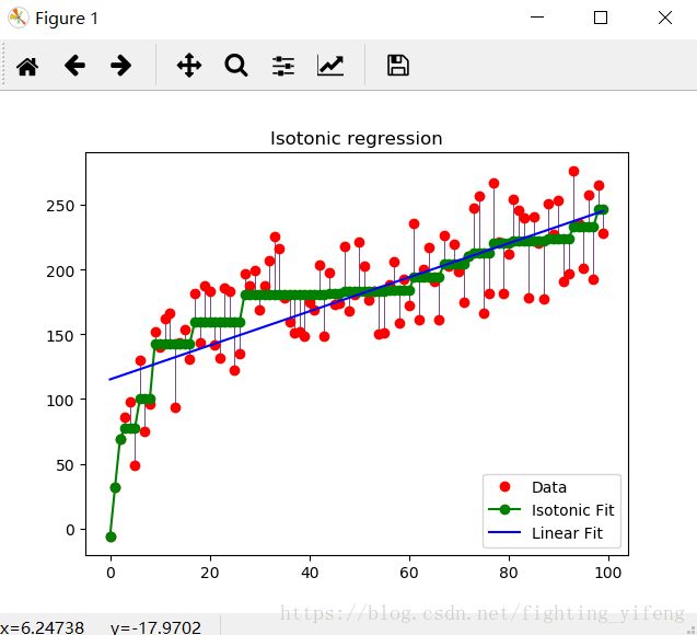
3.sklearn.linear_model.LogisticRegression
print(__doc__)


# Code source: Gaël Varoquaux
# Modified for documentation by Jaques Grobler
# License: BSD 3 clause


import numpy as np
import matplotlib.pyplot as plt

from sklearn import linear_model, decomposition, datasets
from sklearn.pipeline import Pipeline
from sklearn.model_selection import GridSearchCV

logistic = linear_model.LogisticRegression()  #逻辑回归算法。

pca = decomposition.PCA()
pipe = Pipeline(steps=[('pca', pca), ('logistic', logistic)])

digits = datasets.load_digits()
X_digits = digits.data
y_digits = digits.target

# Plot the PCA spectrum
pca.fit(X_digits)

plt.figure(1, figsize=(4, 3))
plt.clf()
plt.axes([.2, .2, .7, .7])
plt.plot(pca.explained_variance_, linewidth=2)
plt.axis('tight')
plt.xlabel('n_components')
plt.ylabel('explained_variance_')

# Prediction
n_components = [20, 40, 64]
Cs = np.logspace(-4, 4, 3)

# Parameters of pipelines can be set using ‘__’ separated parameter names:
estimator = GridSearchCV(pipe,
                         dict(pca__n_components=n_components,
                              logistic__C=Cs))
estimator.fit(X_digits, y_digits)

plt.axvline(estimator.best_estimator_.named_steps['pca'].n_components,
            linestyle=':', label='n_components chosen')
plt.legend(prop=dict(size=12))
plt.show()