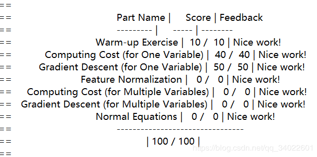
吴恩达机器学习作业讲解（含代码）——ex1(线性回归)

详细代码链接：h5ww

---

Programming Exercise 1: Linear Regression

Files included in this exercise

 你必须要完成以下的函数：

•  warmUpExercise.m - 简单的样例函数
•  plotData.m  - 显示数据集的函数
•  computeCost.m - 线性回归的代价函数
•  gradientDescent.m - 执行梯度下降算法

你可以额外完成以下函数：

• computeCostMulti.m - 多元变量的代价函数
• gradientDescentMulti.m - 多元变量的梯度下降
• featureNormalize.m - 变量正规化
• normalEqn.m - 计算正规方程

---

warmUpExercise.m

要求返回一个5x5的单位向量，文档里给了代码.

% ============= YOUR CODE HERE ==============
% Instructions: Return the 5x5 identity matrix 
%               In octave, we return values by defining which variables
%               represent the return values (at the top of the file)
%               and then set them accordingly. 

A = eye(5);

% ===========================================

---

 plotData.m

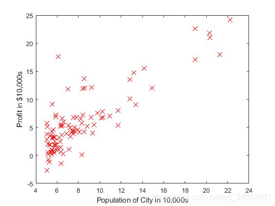
要求在坐标图上画出每个数据点，文档中也同样给出了代码

figure; % 打开新的窗口
% ====================== YOUR CODE HERE ======================
% Instructions: Plot the training data into a figure using the 
%               "figure" and "plot" commands. Set the axes labels using
%               the "xlabel" and "ylabel" commands. Assume the 
%               population and revenue data have been passed in
%               as the x and y arguments of this function.
%
% Hint: You can use the 'rx' option with plot to have the markers
%       appear as red crosses. Furthermore, you can make the
%       markers larger by using plot(..., 'rx', 'MarkerSize', 10);

plot(x,y,'rx','MarkerSize',10);
% plot(x,y,点的样式(r=red,x为叉型),标记大小,设置标记大小为10)
ylabel('Profit in $10,000s');
% 设置y轴标签
xlabel('Population of City in 10,000s');
% 设置x轴标签
% ============================================================

效果：

---

computeCost.m

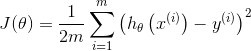
复习一下线性回归的函数：

data = load('ex1data1.txt');
X = data(:, 1); y = data(:, 2);
m = length(y); % number of training examples
...
X = [ones(m, 1), data(:,1)]; % Add a column of ones to x
theta = zeros(2, 1); % initialize fitting parameters
...
% compute and display initial cost
J = computeCost(X, y, theta);

从代码中看出X作为数据矩阵，大小为，y矩阵大小为，theta（）大小为.

我们直接利用线性代数只通过一次矩阵运算直接获得的值。

，直接一步到位等于    ()

 等于

这是矩阵的乘法运算规律，得到的是一个数。

最后这个数除2*m即可。

% ====================== YOUR CODE HERE ======================
% Instructions: Compute the cost of a particular choice of theta
%               You should set J to the cost.
% x*theta get Matrix m*1
x= X*theta-y;
J=(x'*x)/(2*m);
% =========================================================================

---

gradientDescent.m

梯度下降的更新公式：

是学习率（一般取小数），是对求偏导后的结果。

注意的是所有的需要同时更新，同一次迭代中的是不相互影响的。

同样为了运算的直观和方便，也可直接使用矩阵运算，一次运算的到结果。

  是 （）。

要对中每一列都进行一次求内积。然而是一个的列向量，所以先对转置[--]，在和相乘。

结果是

for iter = 1:num_iters

    % ====================== YOUR CODE HERE ======================
    % Instructions: Perform a single gradient step on the parameter vector
    %               theta. 
    %
    % Hint: While debugging, it can be useful to print out the values
    %       of the cost function (computeCost) and gradient here.
    %
 
    x=(alpha*(1/m))*(X'*((X*theta)-y));
    theta=theta-x;
    % ============================================================

    % Save the cost J in every iteration    
    J_history(iter) = computeCost(X, y, theta);

end

---

computeCostMulti.m

多元线性回归的代价函数计算与2元的计算公式 一样。我是利用矩阵运算的，所以不管是多少位变量，都可以一次计算成功。

代码和 computeCost.m 中一样。

% ====================== YOUR CODE HERE ======================
% Instructions: Compute the cost of a particular choice of theta
%               You should set J to the cost.
% x*theta get Matrix m*1
x= X*theta-y;
J=(x'*x)/(2*m);
% =========================================================================

---

gradientDescentMulti.m

矩阵运算优越性就是这样，代码还是一样。

  x=(alpha*(1/m))*(X'*((X*theta)-y));
  theta=theta-x;

---

featureNormalize.m

变量过多也带来了很多问题，不同变量的大小范围是不同的。比如 ，但是在梯度下降更新中学习率一般都是0<<1的，这个导致了在对应的更新很慢。这个导致了整体效率的降低。于是，我们引入变量归一化。归一化的目的是把数变为（0，1）之间的小数。这样我们的更新效率会有所提高。

归一化的公式是：。是被归一化的变量集合，是的平均值，是的标准差或偏差。

这里我们使用标准差。MATLAB中使用mean(x),std(x)分别求均值和标准差。

%遍历X的每一列，对每一列求均值和标准差
%均值存在mu中，标准差存在sigma中，归一化结果存在X_norm中
for i=1:size(X,2)
	mu(i)=mean(X(:,i));
	sigma(i)=std(X(:,i));
	X_norm(:,i)=(X(:,i)-mu(i))/sigma(i);
end

---

normalEqn.m

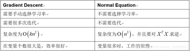
吴恩达在课程中讲过正规方程一步求解最有解的方法。

这个方法通常在X大小适中的时候使用，否在效率会比梯度下降低。

n是指变量的个数。

% ---------------------- Sample Solution ----------------------
theta=pinv((X'*X))*X'*y;
% -------------------------------------------------------------

---