ARIMA模型（p,d,q）参数确定（python）

参数d:

ARIMA 模型对时间序列的要求是平稳型。因此，当你得到一个非平稳的时间序列时，首先要做的即是做时间序列的差分，直到得到一个平稳时间序列。如果你对时间序列做d次差分才能得到一个平稳序列，那么可以使用ARIMA(p,d,q)模型，其中d是差分次数。

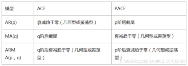
模型的参数p和q由ACF和PACF确定

如下表格

statsmodels介绍

statsmodels（http://www.statsmodels.org）是一个Python库，用于拟合多种统计模型，执行统计测试以及数据探索和可视化。statsmodels包含更多的“经典”频率学派统计方法，而贝叶斯方法和机器学习模型可在其他库中找到。
包含在statsmodels中的一些模型：

• 线性模型，广义线性模型和鲁棒线性模型
• 线性混合效应模型
• 方差分析（ANOVA）方法
• 时间序列过程和状态空间模型
• 广义的矩量法

我们使用其中的时间序列相关函数进行模型的构建。数据为历年美国消费者信心指数数据，代码如下：

%load_ext autoreload
%autoreload 2
%matplotlib inline
%config InlineBackend.figure_format='retina'
import pandas as pd
import numpy as np
import statsmodels.api as sm
import statsmodels.formula.api as smf
import statsmodels.tsa.api as smt
#Display and Plotting
import matplotlib.pylab as plt
import seaborn as sns
# pandas与numpy属性设置
pd.set_option('display.float_format',lambda x:'%.5f'%x)#pandas
np.set_printoptions(precision=5,suppress=True) #numpy
pd.set_option('display.max_columns',100)
pd.set_option('display.max_rows',100)
#seaborn.plotting style
sns.set(style='ticks',context='poster')

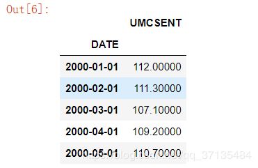
Sentiment='sentiment.csv'
Sentiment=pd.read_csv(Sentiment,index_col=0,parse_dates=[0])

Sentiment.head()

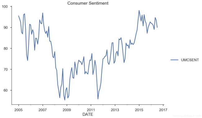
#选取时间断
sentiment_short=Sentiment.loc['2005':'2016']
sentiment_short.plot(figsize=(12,8))
plt.legend(bbox_to_anchor=(1.25,0.5))
plt.title('Consumer Sentiment')
sns.despine()

#help(sentiment_short['UMCSENT'].diff(1))
#函数diss()作用：https://blog.csdn.net/qq_32618817/article/details/80653841#
#https://blog.csdn.net/You_are_my_dream/article/details/70022464,一次差分，和二次差分，减少数据的波动
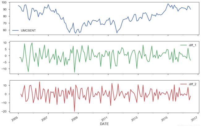
#做一次差分和二次差分（就是在一次差分的结果上再做一次差分）
sentiment_short['diff_1']=sentiment_short['UMCSENT'].diff(1)
sentiment_short['diff_2']=sentiment_short['diff_1'].diff(1)
sentiment_short.plot(subplots=True,figsize=(18,12))

del sentiment_short['diff_2']
del sentiment_short['diff_1']
sentiment_short.head()
print(type(sentiment_short))

自相关函数ACF（Autocorrelation funtion）

• 有序的随机变量序列与其自身相比较，自相关函数反映了同一序列在不同时序的取值之间的相关性
• 公式：$ACF(k)=P_k=\frac{Cov(y_t,y_{t-k})}{Var(y_t)}$
• PK的取值范围为[-1,1]

偏自相关函数（PACF）(partial autocorrelation function)

• 对于一个平稳AR§模型，求出滞后k自相关系数p(k)时 实际上得到并不是x(t)与x(t-k)之间单纯的相关关系
• x(t)同时还会受到中间k-1个随机变量x(t-1)、x(t-2)、……、x(t-k+1)的影响 而这k-1个随机变量又都和x(t-k)具有相关关系 所以自相关系数p(k)里实际掺杂了其他变量对x(t)与x(t-k)的影响
• 剔除了中间k-1个随机变量x(t-1)、x(t-2)、……、x(t-k+1)的干扰之后 x(t-k)对x(t)影响的相关程度
• ACF还包含了其他变量的影响 而偏自相关系数PACF是严格这两个变量之间的相关性

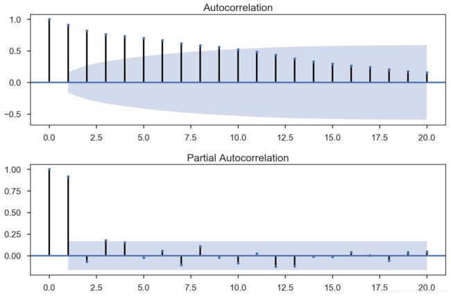
fig=plt.figure(figsize=(12,8))
ax1=fig.add_subplot(211)
fig=sm.graphics.tsa.plot_acf(sentiment_short,lags=20,ax=ax1)#自相关
ax1.xaxis.set_ticks_position('bottom')
fig.tight_layout();
ax2=fig.add_subplot(212)
fig=sm.graphics.tsa.plot_pacf(sentiment_short,lags=20,ax=ax2)#偏自相关
ax2.xaxis.set_ticks_position('bottom')
fig.tight_layout()

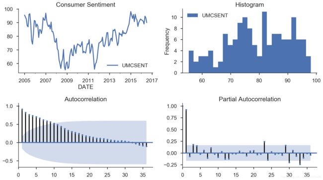
#直观：
def tsplot(y,lags=None,title='',figsize=(14,8)):
    fig=plt.figure(figsize=figsize)
    layout=(2,2)
    ts_ax=plt.subplot2grid(layout,(0,0))
    hist_ax=plt.subplot2grid(layout,(0,1))
    acf_ax=plt.subplot2grid(layout,(1,0))
    pacf_ax=plt.subplot2grid(layout,(1,1))
    y.plot(ax=ts_ax)
    ts_ax.set_title(title)
    y.plot(ax=hist_ax,kind='hist',bins=25)
    hist_ax.set_title('Histogram')
    smt.graphics.plot_acf(y,lags=lags,ax=acf_ax)
    smt.graphics.plot_pacf(y,lags=lags,ax=pacf_ax)
    [ax.set_xlim(0) for ax in [acf_ax, pacf_ax]]
    sns.despine()
    plt.tight_layout()
    #return ts_ax,acf_ax,pacf_ax
tsplot(sentiment_short, title='Consumer Sentiment', lags=36);

参考