1、代码练习
HybridSN 高光谱分类网络
! wget http://www.ehu.eus/ccwintco/uploads/6/67/Indian_pines_corrected.mat
! wget http://www.ehu.eus/ccwintco/uploads/c/c4/Indian_pines_gt.mat
! pip install spectral
import numpy as np
import matplotlib.pyplot as plt
import scipy.io as sio
from sklearn.decomposition import PCA
from sklearn.model_selection import train_test_split
from sklearn.metrics import confusion_matrix, accuracy_score, classification_report, cohen_kappa_score
import spectral
import torch
import torchvision
import torch.nn as nn
import torch.nn.functional as F
import torch.optim as optim
import torch
import torch.nn as nn
import torch.nn.functional as F
import torchvision
import torchvision.transforms as transforms
import matplotlib.pyplot as plt
import numpy as np
import torch.optim as optim
1.定义HybridSN类
#HybridSN类代码
class_num = 16

class HybridSN(nn.Module):
  def __init__(self):
    super(HybridSN, self).__init__()
    self.L = 30
    self.S = 25

    self.conv1 = nn.Conv3d(1, 8, kernel_size=(7, 3, 3), stride=1, padding=0)
    self.conv2 = nn.Conv3d(8, 16, kernel_size=(5, 3, 3), stride=1, padding=0)
    self.conv3 = nn.Conv3d(16, 32, kernel_size=(3, 3, 3), stride=1, padding=0)

    inputX = self.get2Dinput()
    inputConv4 = inputX.shape[1] * inputX.shape[2]
    self.conv4 = nn.Conv2d(inputConv4, 64, kernel_size=(3, 3), stride=1, padding=0)

    num = inputX.shape[3]-2 #二维卷积后(64, 17, 17)-->num = 17
    inputFc1 = 64 * num * num
    self.fc1 = nn.Linear(inputFc1, 256) # 64 * 17 * 17 = 18496
    self.fc2 = nn.Linear(256, 128)
    self.fc3 = nn.Linear(128, class_num)
    self.dropout = nn.Dropout(0.4)

  def get2Dinput(self):
    with torch.no_grad():
      x = torch.zeros((1, 1, self.L, self.S, self.S))
      x = self.conv1(x)
      x = self.conv2(x)
      x = self.conv3(x)
    return x

  def forward(self, x):
    x = F.relu(self.conv1(x))
    x = F.relu(self.conv2(x))
    x = F.relu(self.conv3(x))
    x = x.view(x.shape[0], -1, x.shape[3], x.shape[4])
    x = F.relu(self.conv4(x))
    x = x.view(-1, x.shape[1] * x.shape[2] * x.shape[3])
    x = F.relu(self.fc1(x))
    x = self.dropout(x)
    x = F.relu(self.fc2(x))
    x = self.dropout(x)
    x = self.fc3(x)
    return x

# 随机输入,测试网络结构是否通
# x = torch.randn(1, 1, 30, 25, 25)
# net = HybridSN()
# y = net(x)
# print(y.shape)
2.创建数据集
#定义基本函数
# 对高光谱数据 X 应用 PCA 变换
def applyPCA(X, numComponents):
    newX = np.reshape(X, (-1, X.shape[2]))
    pca = PCA(n_components=numComponents, whiten=True)
    newX = pca.fit_transform(newX)
    newX = np.reshape(newX, (X.shape[0], X.shape[1], numComponents))
    return newX

# 对单个像素周围提取 patch 时,边缘像素就无法取了,因此,给这部分像素进行 padding 操作
def padWithZeros(X, margin=2):
    newX = np.zeros((X.shape[0] + 2 * margin, X.shape[1] + 2* margin, X.shape[2]))
    x_offset = margin
    y_offset = margin
    newX[x_offset:X.shape[0] + x_offset, y_offset:X.shape[1] + y_offset, :] = X
    return newX

# 在每个像素周围提取 patch ,然后创建成符合 keras 处理的格式
def createImageCubes(X, y, windowSize=5, removeZeroLabels = True):
    # 给 X 做 padding
    margin = int((windowSize - 1) / 2)
    zeroPaddedX = padWithZeros(X, margin=margin)
    # split patches
    patchesData = np.zeros((X.shape[0] * X.shape[1], windowSize, windowSize, X.shape[2]))
    patchesLabels = np.zeros((X.shape[0] * X.shape[1]))
    patchIndex = 0
    for r in range(margin, zeroPaddedX.shape[0] - margin):
        for c in range(margin, zeroPaddedX.shape[1] - margin):
            patch = zeroPaddedX[r - margin:r + margin + 1, c - margin:c + margin + 1]
            patchesData[patchIndex, :, :, :] = patch
            patchesLabels[patchIndex] = y[r-margin, c-margin]
            patchIndex = patchIndex + 1
    if removeZeroLabels:
        patchesData = patchesData[patchesLabels>0,:,:,:]
        patchesLabels = patchesLabels[patchesLabels>0]
        patchesLabels -= 1
    return patchesData, patchesLabels

def splitTrainTestSet(X, y, testRatio, randomState=345):
    X_train, X_test, y_train, y_test = train_test_split(X, y, test_size=testRatio, random_state=randomState, stratify=y)
    return X_train, X_test, y_train, y_test
#读取并创建数据集
# 地物类别
class_num = 16
X = sio.loadmat('Indian_pines_corrected.mat')['indian_pines_corrected']
y = sio.loadmat('Indian_pines_gt.mat')['indian_pines_gt']
# 用于测试样本的比例
test_ratio = 0.90
# 每个像素周围提取 patch 的尺寸
patch_size = 25
# 使用 PCA 降维,得到主成分的数量
pca_components = 30
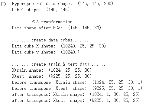
print('Hyperspectral data shape: ', X.shape)
print('Label shape: ', y.shape)
print('\n... ... PCA tranformation ... ...')
X_pca = applyPCA(X, numComponents=pca_components)
print('Data shape after PCA: ', X_pca.shape)
print('\n... ... create data cubes ... ...')
X_pca, y = createImageCubes(X_pca, y, windowSize=patch_size)
print('Data cube X shape: ', X_pca.shape)
print('Data cube y shape: ', y.shape)
print('\n... ... create train & test data ... ...')
Xtrain, Xtest, ytrain, ytest = splitTrainTestSet(X_pca, y, test_ratio)
print('Xtrain shape: ', Xtrain.shape)
print('Xtest shape: ', Xtest.shape)
# 改变 Xtrain, Ytrain 的形状,以符合 keras 的要求
Xtrain = Xtrain.reshape(-1, patch_size, patch_size, pca_components, 1)
Xtest = Xtest.reshape(-1, patch_size, patch_size, pca_components, 1)
print('before transpose: Xtrain shape: ', Xtrain.shape)
print('before transpose: Xtest shape: ', Xtest.shape)
# 为了适应 pytorch 结构,数据要做 transpose
Xtrain = Xtrain.transpose(0, 4, 3, 1, 2)
Xtest = Xtest.transpose(0, 4, 3, 1, 2)
print('after transpose: Xtrain shape: ', Xtrain.shape)
print('after transpose: Xtest shape: ', Xtest.shape)
""" Training dataset"""
class TrainDS(torch.utils.data.Dataset):
def __init__(self):
self.len = Xtrain.shape[0]
self.x_data = torch.FloatTensor(Xtrain)
self.y_data = torch.LongTensor(ytrain)
def __getitem__(self, index):
# 根据索引返回数据和对应的标签
return self.x_data[index], self.y_data[index]
def __len__(self):
# 返回文件数据的数目
return self.len
""" Testing dataset"""
class TestDS(torch.utils.data.Dataset):
def __init__(self):
self.len = Xtest.shape[0]
self.x_data = torch.FloatTensor(Xtest)
self.y_data = torch.LongTensor(ytest)
def __getitem__(self, index):
# 根据索引返回数据和对应的标签
return self.x_data[index], self.y_data[index]
def __len__(self):
# 返回文件数据的数目
return self.len
# 创建 trainloader 和 testloader
trainset = TrainDS()
testset = TestDS()
train_loader = torch.utils.data.DataLoader(dataset=trainset, batch_size=128, shuffle=True, num_workers=2)
test_loader = torch.utils.data.DataLoader(dataset=testset, batch_size=128, shuffle=False, num_workers=2)
3.开始训练
# 使用GPU训练,可以在菜单 "代码执行工具" -> "更改运行时类型" 里进行设置
device = torch.device("cuda:0" if torch.cuda.is_available() else "cpu")
# 网络放到GPU上
net = HybridSN().to(device)
criterion = nn.CrossEntropyLoss()
optimizer = optim.Adam(net.parameters(), lr=0.001)
# 开始训练
total_loss = 0
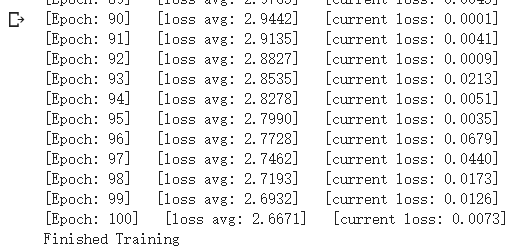
for epoch in range(100):
for i, (inputs, labels) in enumerate(train_loader):
inputs = inputs.to(device)
labels = labels.to(device)
# 优化器梯度归零
optimizer.zero_grad()
# 正向传播 + 反向传播 + 优化
outputs = net(inputs)
loss = criterion(outputs, labels)
loss.backward()
optimizer.step()
total_loss += loss.item()
print('[Epoch: %d] [loss avg: %.4f] [current loss: %.4f]' %(epoch + 1, total_loss/(epoch+1), loss.item()))
print('Finished Training')
4.模型测试
count = 0
# 模型测试
for inputs, _ in test_loader:
inputs = inputs.to(device)
outputs = net(inputs)
outputs = np.argmax(outputs.detach().cpu().numpy(), axis=1)
if count == 0:
y_pred_test = outputs
count = 1
else:
y_pred_test = np.concatenate( (y_pred_test, outputs) )
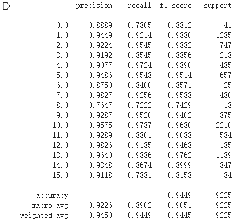
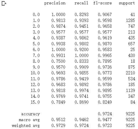
# 生成分类报告
classification = classification_report(ytest, y_pred_test, digits=4)
print(classification)
5.备用函数
#用于计算各个类准确率,显示结果的备用函数
from operator import truediv

def AA_andEachClassAccuracy(confusion_matrix):
    counter = confusion_matrix.shape[0]
    list_diag = np.diag(confusion_matrix)
    list_raw_sum = np.sum(confusion_matrix, axis=1)
    each_acc = np.nan_to_num(truediv(list_diag, list_raw_sum))
    average_acc = np.mean(each_acc)
    return each_acc, average_acc


def reports (test_loader, y_test, name):
    count = 0
    # 模型测试
    for inputs, _ in test_loader:
        inputs = inputs.to(device)
        outputs = net(inputs)
        outputs = np.argmax(outputs.detach().cpu().numpy(), axis=1)
        if count == 0:
            y_pred =  outputs
            count = 1
        else:
            y_pred = np.concatenate( (y_pred, outputs) )

    if name == 'IP':
        target_names = ['Alfalfa', 'Corn-notill', 'Corn-mintill', 'Corn'
                        ,'Grass-pasture', 'Grass-trees', 'Grass-pasture-mowed',
                        'Hay-windrowed', 'Oats', 'Soybean-notill', 'Soybean-mintill',
                        'Soybean-clean', 'Wheat', 'Woods', 'Buildings-Grass-Trees-Drives',
                        'Stone-Steel-Towers']
    elif name == 'SA':
        target_names = ['Brocoli_green_weeds_1','Brocoli_green_weeds_2','Fallow','Fallow_rough_plow','Fallow_smooth',
                        'Stubble','Celery','Grapes_untrained','Soil_vinyard_develop','Corn_senesced_green_weeds',
                        'Lettuce_romaine_4wk','Lettuce_romaine_5wk','Lettuce_romaine_6wk','Lettuce_romaine_7wk',
                        'Vinyard_untrained','Vinyard_vertical_trellis']
    elif name == 'PU':
        target_names = ['Asphalt','Meadows','Gravel','Trees', 'Painted metal sheets','Bare Soil','Bitumen',
                        'Self-Blocking Bricks','Shadows']

    classification = classification_report(y_test, y_pred, target_names=target_names)
    oa = accuracy_score(y_test, y_pred)
    confusion = confusion_matrix(y_test, y_pred)
    each_acc, aa = AA_andEachClassAccuracy(confusion)
    kappa = cohen_kappa_score(y_test, y_pred)

    return classification, confusion, oa*100, each_acc*100, aa*100, kappa*100
#检测结果写在文件里
classification, confusion, oa, each_acc, aa, kappa = reports(test_loader, ytest, 'IP')
classification = str(classification)
confusion = str(confusion)
file_name = "classification_report.txt"

with open(file_name, 'w') as x_file:
    x_file.write('\n')
    x_file.write('{} Kappa accuracy (%)'.format(kappa))
    x_file.write('\n')
    x_file.write('{} Overall accuracy (%)'.format(oa))
    x_file.write('\n')
    x_file.write('{} Average accuracy (%)'.format(aa))
    x_file.write('\n')
    x_file.write('\n')
    x_file.write('{}'.format(classification))
    x_file.write('\n')
    x_file.write('{}'.format(confusion))
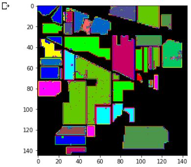
#显示分类结果
# load the original image
X = sio.loadmat('Indian_pines_corrected.mat')['indian_pines_corrected']
y = sio.loadmat('Indian_pines_gt.mat')['indian_pines_gt']
height = y.shape[0]
width = y.shape[1]
X = applyPCA(X, numComponents= pca_components)
X = padWithZeros(X, patch_size//2)
# 逐像素预测类别
outputs = np.zeros((height,width))
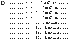
for i in range(height):
for j in range(width):
if int(y[i,j]) == 0:
continue
else :
image_patch = X[i:i+patch_size, j:j+patch_size, :]
image_patch = image_patch.reshape(1,image_patch.shape[0],image_patch.shape[1], image_patch.shape[2], 1)
X_test_image = torch.FloatTensor(image_patch.transpose(0, 4, 3, 1, 2)).to(device)
prediction = net(X_test_image)
prediction = np.argmax(prediction.detach().cpu().numpy(), axis=1)
outputs[i][j] = prediction+1
if i % 20 == 0:
print('... ... row ', i, ' handling ... ...')
predict_image = spectral.imshow(classes = outputs.astype(int),figsize =(5,5))
SENet实现
class SELayer(nn.Module):
  def __init__(self,channel,reduction=16):
    super(SELayer,self).__init__()
    self.avg_pool = nn.AdaptiveAvgPool2d(1)
    self.fc = nn.Sequential(
        nn.Linear(channel,channel//reduction,bias=False),
        nn.ReLU(inplace=True),
        nn.Linear(channel//reduction,channel,bias=False),
        nn.Sigmoid()
    )
  def forward(self,x):
    b,c,_,_ = x.size()
    y = self.avg_pool(x).view(b,c)
    y = self.fc(y).view(b,c,1,1)
    return x*y.expand_as(x)

class HybridSN(nn.Module):
  def __init__(self,reduction=16):
    super(HybridSN, self).__init__()
    self.L = 30
    self.S = 25

    self.conv1 = nn.Conv3d(1, 8, kernel_size=(7, 3, 3), stride=1, padding=0)
    self.conv2 = nn.Conv3d(8, 16, kernel_size=(5, 3, 3), stride=1, padding=0)
    self.conv3 = nn.Conv3d(16, 32, kernel_size=(3, 3, 3), stride=1, padding=0)

    inputX = self.get2Dinput()
    inputConv4 = inputX.shape[1] * inputX.shape[2]
    self.conv4 = nn.Conv2d(inputConv4, 64, kernel_size=(3, 3), stride=1, padding=0)

    num = inputX.shape[3]-2 #二维卷积后(64, 17, 17)-->num = 17
    inputFc1 = 64 * num * num
    self.se = SELayer(64,reduction)
    self.fc1 = nn.Linear(inputFc1, 256) # 64 * 17 * 17 = 18496
    self.fc2 = nn.Linear(256, 128)
    self.fc3 = nn.Linear(128, class_num)
    self.dropout = nn.Dropout(0.4)

  def get2Dinput(self):
    with torch.no_grad():
      x = torch.zeros((1, 1, self.L, self.S, self.S))
      x = self.conv1(x)
      x = self.conv2(x)
      x = self.conv3(x)
    return x

  def forward(self, x):
    x = F.relu(self.conv1(x))
    x = F.relu(self.conv2(x))
    x = F.relu(self.conv3(x))
    x = x.view(x.shape[0], -1, x.shape[3], x.shape[4])
    x = F.relu(self.conv4(x))
    x = x.view(-1, x.shape[1] * x.shape[2] * x.shape[3])
    x = F.relu(self.fc1(x))
    x = self.se(x)
    x = self.dropout(x)
    x = F.relu(self.fc2(x))
    x = self.dropout(x)
    x = self.fc3(x)
    return x
# 随机输入,测试网络结构是否通
# x = torch.randn(1, 1, 30, 25, 25)
# net = HybridSN()
# y = net(x)
# print(y.shape)
· 精度与之前相比有所提升。
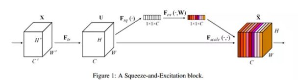
· 传统的方法是将网络的Feature Map等权重的传到下一层,SENet的核心思想在于建模通道之间的相互依赖关系,通过网络的全局损失函数自适应的重新矫正通道之间的特征相应强度。
· SENet由一些列SE block组成,一个SE block的过程分为Squeeze(压缩)和Excitation(激发)两个步骤。
○ Squeeze通过在Feature Map层上执行Global Average Pooling得到当前Feature Map的全局压缩特征向量。
○ Excitation通过两层全连接得到Feature Map中每个通道的权值,并将加权后的Feature Map作为下一层网络的输入。
· SE block只依赖与当前的一组Feature Map,因此可以非常容易的嵌入到几乎现在所有的卷积网络中。
一个SE Block如下图所示
2、视频学习
《语义分割中的自注意力机制和低秩重重建》——北京大学李夏
什么是语义分割?
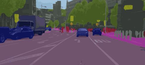
语义分割是计算机视觉领域的一项基础任务,它的目标是为每个像素预测类别标签。由于类别多样繁杂,且类间表征相似度大,语义分割要求模型具有强大的区分能力。近年来,基于全卷积网络(FCN[1])的一系列研究,在该任务上取得了卓越的成绩。
在语义分割中我们需要将视觉输入分为不同的语义可解释类别,「语义的可解释性」即分类类别在真实世界中是有意义的。例如,我们可能需要区分图像中属于汽车的所有像素,并把这些像素涂成蓝色。
· 图像分类任务:对每个图像输出一个label。
· 语义分割任务:对图像中的每一个像素输出一个label(对每一个像素点定义一个类别),并且输出是同时的,语义分割需要非常大的感知域。
与图像分类或目标检测相比,语义分割使我们对图像有更加细致的了解。这种了解在诸如自动驾驶、机器人以及图像搜索引擎等许多领域都是非常重要的。
Attention机制
Attention机制的本质:
Attention机制源自于人类视觉注意力机制:将有限的注意力集中在重点信息上,「从关注全部到关注重点」,所谓Attention机制,便是聚焦于局部信息的机制,从而节省资源,快速获得最有效的信息。
对于Attention而言,就是一种权重参数的分配机制,目标是协助模型捕捉重要信息。
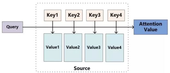
Attention的原理
可以将attention机制看做一种query机制,即用一个query来检索一个memory区域。我们将query表示为key_q,memory是一个键值对集合(a set of key-value pairs),共有M项,其中的第i项我们表示为
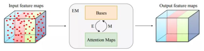
期望最大化注意力机制(EMA)
本文所提出的期望最大化注意力机制(EMA),摒弃了在全图上计算注意力图的流程,转而通过期望最大化(EM)算法迭代出一组紧凑的基,在这组基上运行注意力机制,从而大大降低了复杂度。其中,E 步更新注意力图,M 步更新这组基。E、M 交替执行,收敛之后用来重建特征图。本文把这一机制嵌入网络中,构造出轻量且易实现的 EMA Unit。其作为语义分割头,在多个数据集上取得了较高的精度。
期望最大化注意力模块(EMA Unit)
期望最大化注意力模块(EMAU)的结构如图所示。除了核心的 EMA 之外,两个 1×1 卷积分别放置于 EMA 前后。前者将输入的值域从 R+映射到 R;后者将 X tilde 映射到 X 的残差空间。囊括进两个卷积的额外负荷,EMAU 的 FLOPs 仅相当于同样输入输出大小时 3×3 卷积的 1/3,参数量仅为 2C^2+KC。

《图像语义分割前沿进展》——南开大学程明明教授
·图像分割领域数据集
当前图像分割领域使用的主要有Pascol VOC、CityScapes、COCO Stuff等数据集
大的数据集对图像分割领域是有一定的帮助的,至于帮助有多大,在这个数据集出来之前是没办法预测的
但是无论数据集有多大,都会存在一个长尾问题
怎么样利用好一些没有标注的数据是一个比较好的研究方向
·弱监督图像语义分割
图像分割的任务是对每个像素都进行标注。因此,在深度学习方法中,直观上就需要所有的像素都有真值标注。在这个要求下,真值标注的生成是极度耗时耗力的,尤其是以人工标注的方式。比如,CityScapes数据库,在精标条件下,一张图片的标注就需要1.5个小时。如此一来,数据库标注的成本可想而知。基于此,许多研究人员就想到用弱监督的方式进行网络训练,从而降低标注成本。
常见的输入有image-level tags和bounding boxes
弱监督图像语义分割在最近几年进展较快,它只依赖于图像类别标签等轻量级标注数据,正在成为学术界研究的热点。
Note:
当前的一些图像分割算法可能存在着计算量、小物体分割等方面的一些问题,考虑从哪方面进行改进和突破时,可以尽量结合自己擅长的方向寻找突破点,不一定非要另辟蹊径。
对于某种方式方法讨论它的应用有哪些,应该从应用的角度考虑应用,要结合应用的实际情况,比如某项指标达到90%,在实际应用中不一定90%的情况都会有对。不同应用差距很大。
·图像分割领域技术未来重要发展方向和研究问题
○ AutoML
○ 轻量级模型设计
○ Attention机制
○ 视频分割
对于一个领域的发展,应该鼓励百花齐放,百花争鸣。从不同的角度思考,会有不同的看法。