数值计算详细笔记（三）：线性方程组解法

6. Linear Systems Ax = b

6.1 Basic Concepts

6.1.1 LSEs

the Linear System of Equations (LSEs):
$$(I)\{\begin{array}{rl}{E}_1:& a_{11}{x}_1+a_{12}{x}_2+...+a_{1n}{x}_n=b_1\\ E_2:& a_{21}{x}_1+a_{22}{x}_2+...+a_{2n}{x}_n=b_2\\ ...& \\ E_n:& a_{n1}{x}_1+a_{n2}{x}_2+...+a_{nn}{x}_n=b_n\end{array}$$

6.1.2 Operations of LSEs

Multiplied operation - 数乘

Equation $E_i$ can be multiplied by any nonzero constant $\lambda$
$$(\lambda E_i)\to E_i$$

Multiplied and added operation - 倍加

Equation $E_j$ can be multiplied by any nonzero constant $\lambda$, and added to Equation $E_i$ in place of $E_i$, denoted by
$$(\lambda E_j+E_i)\to E_i$$

Transposition - 交换

Equation $E_i$ and $E_j$ can be transposed in order, denoted by
$$E_i\leftrightarrow E_j$$

6.1.3 Augmented Matirx

$$\tilde{A}=[A,\text{b}]=\left(\begin{array}{cc}\begin{array}{cccc}{a}_{11}& a_{12}& ...& a_{1n}\\ a_{21}& a_{22}& ...& a_{2n}\\ ...& ...& ...& ...\\ a_{n1}& a_{n2}& ...& a_{nn}\end{array}& \begin{array}{c}{b}_1\\ b_2\\ ...\\ b_n\end{array}\end{array}\right)$$

6.2 Gaussian Elimination Method

6.2.1 Overall Description

The key point of Gaussian Elimination Method is changing the original matrix into upper-triangular matrix, then using backward–substitution method to calculate the answer.

6.2.2 Algorithm

• INPUT: $N$-dimension, $A(N,N),B(N)$

• OUTPUT: Solution $x(N)$ or Message that LESs has no unique solution.

• Step $1$: For $k=1,2,...,N-1$, do step 2-4.

• Step $2$: Set $p$ be the smallest integer with $k\le p\le N$ and $A_{p,k}\ne 0$. If no $p$ can be found, output: “no unique solution exists”; stop.

• Step $3$: If $p\ne k$, do transposition $E_p\leftrightarrow E_k$.

• Step $4$: For $i=k+1,...,N$

  1. Set $m_{i,k}=\frac{A(i,k)}{A(k,k)}$
  2. Set $B(i)=B(i)-m_{i,k}B(k)$
  3. For $j=k+1,...,N$, set $A(i,j)=A(i,j)-m_{i,k}A(k,j)$;

• Step $5$: If $A(N,N)\ne 0$, set $x(N)=\frac{B(N)}{A(N,N)}$; Else, output:“no unique solution exists.”

• Step $6$: For $i=N-1,N-2,...,1$, set
  $$X(i)=[B(i)-\sum _{j=i+1}^{N}A(i,j)x(j)]/A(i,i)$$

• Step $7$: Output the solution $x(N)$.

6.3 Pivoting Strategies

6.3.1 Background

According to the process of Gaussian Elimination Method, We find that if $a_{kk}^{(k-1)}$ is too small, the roundoff error will be larger.
$$\begin{gathered} m_{i,k}=\frac{A(i,k)}{A(k,k)} \\ X(i)=[B(i)-\sum _{j=i+1}^{N}A(i,j)x(j)]/A(i,i) \end{gathered}$$

Therefore, in order to reduce the roundoff error, we need to make the value of $a_{kk}^{(k-1)}$ larger.

6.3.2 Maximal Column Pivoting Technique

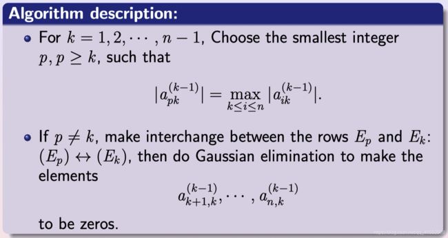
This method is to make $a_{kk}^{(k-1)}$ equal to the maximal value in its column.

6.3.3 Maximal Row Pivoting Technique

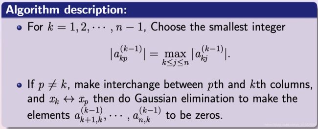
This method is to make $a_{kk}^{(k-1)}$ equal to the maximal value in its row.

6.3.4 Partial Pivoting Technique

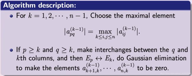
This method is to make $a_{kk}^{(k-1)}$ equal to the maximal value in its remaining area.

6.3.5 Scaled Partial Pivoting Technique

$$\begin{gathered} s_i=\underset{1\le j\le n}{\max }|a_{i,j}| \\ \frac{a_{kk}}{s_k}=\underset{k\le i\le n}{\max }\frac{a_{i,1}}{s_i} \end{gathered}$$

This method is to make $\frac{a_{kk}^{(k-1)}}{s_k}$ equal to the maximal value in its remaining area.

6.4 LU Factorization

6.4.1 The advantage of LU Factorization

$$\begin{gathered} Ax=b \\ A=LU \\ L=\left(\begin{array}{ccccc}1& 0& 0& ...& 0\\ l_{21}& 1& 0& ...& 0\\ l_{31}& l_{32}& 1& ...& 0\\ ...& ...& ...& ...& ...\\ l_{n1}& l_{n2}& l_{n3}& ...& 1\end{array}\right),R=\left(\begin{array}{ccccc}{u}_{11}& u_{12}& u_{13}& ...& u_{1n}\\ 0& u_{22}& u_{23}& ...& u_{2n}\\ 0& 0& u_{33}& ...& u_{3n}\\ ...& ...& ...& ...& ...\\ 0& 0& 0& ...& u_{nn}\end{array}\right) \end{gathered}$$

We can use two-step process to solve $LUx=b$.

1. $y=Ux,Ly=b$
2. Solve $Ly=b$ determining $y$ with forward substitution method.
3. Solve $Ux=y$ determining $x$ with forward substitution method.

6.4.2 LU Factorization through Gaussian Elimination

Theorem

If Gaussian elimination can be performed on the linear system $Ax=b$ without row interchanges, then the matrix $A$ can be factored into the product of a lower-triangular $L$ and an upper-triangular matrix $U$,
$$A=LU$$
where
$$L=\left(\begin{array}{ccccc}1& 0& 0& ...& 0\\ m_{21}& 1& 0& ...& 0\\ m_{31}& m_{32}& 1& ...& 0\\ ...& ...& ...& ...& ...\\ m_{n1}& m_{n2}& m_{n3}& ...& 1\end{array}\right),R=\left(\begin{array}{ccccc}{a}_{11}^1& a_{12}^1& a_{13}^1& ...& a_{1n}^1\\ 0& a_{22}^2& a_{23}^2& ...& a_{2n}^2\\ 0& 0& a_{33}^3& ...& a_{3n}^3\\ ...& ...& ...& ...& ...\\ 0& 0& 0& ...& a_{nn}^n\end{array}\right)$$

Proof

$$\begin{gathered} m_{j,1}=\frac{a_{j,1}}{a_{1,1}} \\ {M}^1=\left(\begin{array}{ccccc}1& 0& 0& ...& 0\\ -m_{21}& 1& 0& ...& 0\\ -m_{31}& 0& 1& ...& 0\\ ...& ...& ...& ...& ...\\ -m_{n1}& 0& 0& ...& 1\end{array}\right) \end{gathered}$$
Thus,
$$A^n=M^{n-1}{M}^{n-2}...M^{1}A.$$
Let $U=A^n$, then
$$\begin{gathered} [M^1{]}^{-1}...[M^{n-2}{]}^{-1}[M^{n-1}{]}^{-1}U=A \\ [M^1{]}^{-1}=\left(\begin{array}{ccccc}1& 0& 0& ...& 0\\ m_{21}& 1& 0& ...& 0\\ m_{31}& 0& 1& ...& 0\\ ...& ...& ...& ...& ...\\ m_{n1}& 0& 0& ...& 1\end{array}\right) \\ L=[M^1{]}^{-1}...[M^{n-2}{]}^{-1}[M^{n-1}{]}^{-1} \end{gathered}$$

6.4.3 LU Factorization through Gaussian Elimination

$$\begin{gathered} LU=\left(\begin{array}{ccccc}1& 0& 0& ...& 0\\ l_{21}& 1& 0& ...& 0\\ l_{31}& l_{32}& 1& ...& 0\\ ...& ...& ...& ...& ...\\ l_{n1}& l_{n2}& l_{n3}& ...& 1\end{array}\right)\left(\begin{array}{ccccc}{u}_{11}& u_{12}& u_{13}& ...& u_{1n}\\ 0& u_{22}& u_{23}& ...& u_{2n}\\ 0& 0& u_{33}& ...& u_{3n}\\ ...& ...& ...& ...& ...\\ 0& 0& 0& ...& u_{nn}\end{array}\right) \\ LU=A=\left(\begin{array}{ccccc}{a}_{11}& a_{12}& a_{13}& ...& a_{1n}\\ a_{21}& a_{22}& a_{23}& ...& a_{2n}\\ a_{31}& a_{32}& a_{33}& ...& a_{3n}\\ ...& ...& ...& ...& ...\\ a_{n1}& a_{n2}& a_{n3}& ...& a_{nn}\end{array}\right) \end{gathered}$$

Algorithm

6.5 Strictly Diagonally dominant Matrix

6.5.1 Definition

The $n\ast n$ matrix is said to be strictly diagonally dominant (严格对角占优) when
$$|a_{ii}|>\sum _{j=1,j\ne i}^n|a_{ij}|$$
holds for each $i=1,2,3,...,n$.

6.5.2 Property

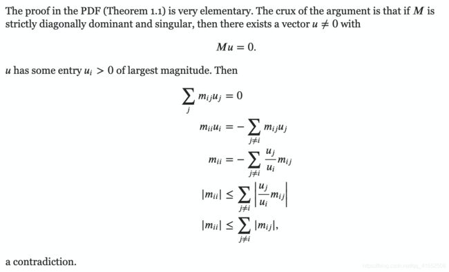
1. A strictly diagonally dominant matrix $A$ is nonsingular.
2. Moreover, in this case, Gaussian elimination can be performed on any linear system of the form $Ax=b$ to obtain its unique solution without row or column interchanges, and the computations are stable with respect to the growth of roundoff errors.

Proof for First Property

A matrix is singular means its determinant is zero.

A matrix’s determinant is zero means the n vectors in the matrix are linearly dependent.

Thus, matrix $A$ is singular means there exists a column vector $u$ that $Ax=0$.

6.6 Positive Definite Symmetric Matrix

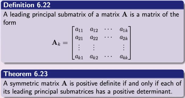
6.6.1 Definition

A matrix $A$ is positive definite if it is symmetric and if $x^{T}Ax>0$ for every $n$-dimensional column vector $x\ne 0$.

6.6.2 Property

If A is an $n\ast n$ positive definite matrix, then

1. A is nonsingular;
2. $a_{ii}>0$ for each $i=1,2,...,n$;
3. ${\max }_{1\le k,j\le n}|a_{k,j}|\le {\max }_{1\le i\le n}|a_{i,i}|$;
4. $a_{ij}^2<a_{ii}{a}_{jj}$ for each $i\ne j$.

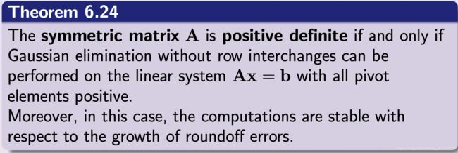
6.6.3 Theorem

6.7 $L{L}^T$ Factorization

6.7.1 Definition

For a $n\ast n$ symmetric and positive definite matrix $A$ with the form
$$A=\left(\begin{array}{ccccc}{a}_{11}& a_{12}& a_{13}& ...& a_{1n}\\ a_{12}& a_{22}& a_{23}& ...& a_{2n}\\ a_{13}& a_{23}& a_{33}& ...& a_{3n}\\ ...& ...& ...& ...& ...\\ a_{1n}& a_{2n}& a_{3n}& ...& a_{nn}\end{array}\right)$$
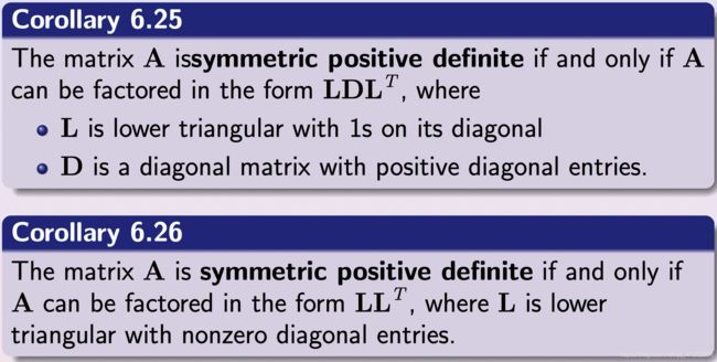
where $A^T=A.$ We can factorize this matrix to the form like $L{L}^T=A$, where $L$ is a lower triangular matrix with form as follows
$$\left(\begin{array}{ccccc}{l}_{11}& 0& 0& \cdots & 0\\ l_{21}& l_{22}& 0& \cdots & 0\\ l_{31}& l_{32}& l_{33}& \cdots & 0\\ ⋮& ⋮& ⋮& \ddots & ⋮\\ l_{n1}& l_{n2}& l_{n3}& \cdots & l_{nn}\end{array}\right)$$

Thus, we need to determine the elements $l_{ij}$, for $i\in [1,n]$ and $j\in [1,n]$.
$$A=\left(\begin{array}{ccccc}{a}_{11}& a_{12}& a_{13}& ...& a_{1n}\\ a_{12}& a_{22}& a_{23}& ...& a_{2n}\\ a_{13}& a_{23}& a_{33}& ...& a_{3n}\\ ...& ...& ...& ...& ...\\ a_{1n}& a_{2n}& a_{3n}& ...& a_{nn}\end{array}\right)=L{L}^T$$

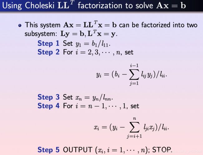
6.7.2 Choleski’s Algorithm

Calculate the value one row by one row

To factor the positive definite $n\ast n$ matrix $A$ into $L{L}^T$, where $L$ is lower triangular:

• INPUT: the dimension $n$; entries $a_{ij}$ of $A$, for $i\in [1,n]$ and $j\in [1,i]$.

• OUTPUT: the entries $l_{ij}$ of $L$, for $i\in [1,n]$ and $j\in [1,i]$.

• Step $1$: Set $l_{11}=\sqrt{a_{11}}$.

• Step $2$: For $j\in [2,n]$, set $l_{j1}=\frac{a_{1j}}{l_{11}}$

• Step $3$: For $i\in [2,n-1]$, do Steps 4 and 5.

• Step $4$: Set $l_{ii}=[a_{ii}-{\sum }_{j=1}^{i-1}{l}_{ij}^2{]}^{\frac{1}{2}}$.

• Step $5$: For $j\in [i+1,n]$, set $l_{ji}=\frac{a_{ij}-{\sum }_{k=1}^{i-1}{l}_{ik}{l}_{jk}}{l_{ii}}$

• Step $6$: Set $l_{nn}=[a_{nn}-{\sum }_{k=1}^{n-1}{l}_{nk}^2{]}^{\frac{1}{2}}$

• Step $7$: OUTPUT $l_{ij}$ for $j\in [1,i]$ and $i\in [1,n]$. STOP!

Example

6.8 $LD{L}^T$ Factorization

6.8.1 Definition

Matrix $A$ is a positive definite matrix, thus
$$A=LD{L}^T.$$

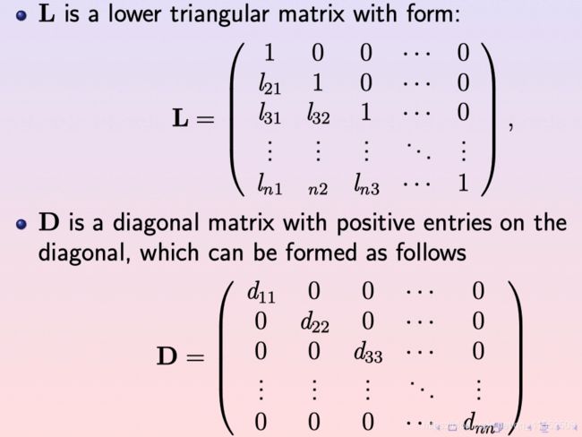
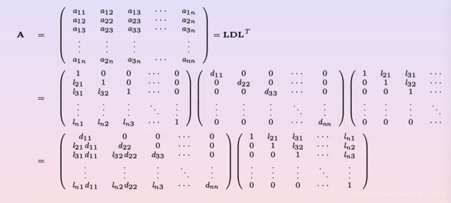
We can calculate the value of $L$ and $D$ one row by one row.

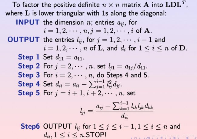
6.8.2 Algorithm

6.9 Tri-diagonal Linear System

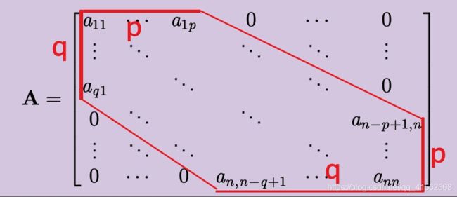
6.9.1 Definition

An $n\ast n$ matrix $A$ is called a band matrix (带状矩阵), if integers $p$ and $q$, with $1<p,q<n$, exist having the property that $a_{ij}=0$ whenever $i+p\le j$ or $j+q\le i$. The bandwidth (带宽) of a band matrix is defined as $w=p+q-1$.

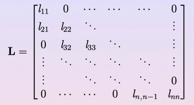
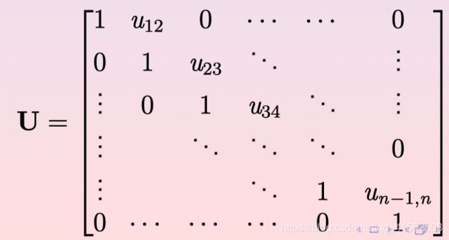
6.9.2 LU Factorization

$$A=LU$$

In order to solve the problem of $Ax=LUx=b$, there are two steps to do.

1. $z=Ux$, and solve $Lz=b$
2. solve $Ux=z$

6.9.3 Remarks

1. Band matrices usually are sparse matrices, thus we need to substitute two-dimensional array to one-dimensional array to store the value of the matrices.
2. Banded matrices appear in numerical calculation methods of partial differential equations and are common matrix forms.