clear
% http://www.peteryu.ca/tutorials/matlab/visualize_decision_boundaries
% load RankData
% NumTrain =200;
load RankData2
% X = [X, -ones(size(X,1),1)];
lambda = 20;
rho = 2;
c1 =10;
c2 =10;
epsilon = 0.2;
result=[];
ker = 'linear';
ker = 'rbf';
sigma = 1/200;
method=4
contour_level1 = [-epsilon,0, epsilon];
contour_level2 = [-epsilon,0, epsilon];
xrange = [-5 5];
yrange = [-5 5];
% step size for how finely you want to visualize the decision boundary.
inc = 0.1;
% generate grid coordinates. this will be the basis of the decision
% boundary visualization.
[x1, x2] = meshgrid(xrange(1):inc:xrange(2), yrange(1):inc:yrange(2));
% size of the (x, y) image, which will also be the size of the
% decision boundary image that is used as the plot background.
image_size = size(x1)
xy = [x1(:) x2(:)]; % make (x,y) pairs as a bunch of row vectors.
%xy = [reshape(x, image_size(1)*image_size(2),1) reshape(y, image_size(1)*image_size(2),1)]
% loop through each class and calculate distance measure for each (x,y)
% from the class prototype.
% calculate the city block distance between every (x,y) pair and
% the sample mean of the class.
% the sum is over the columns to produce a distance for each (x,y)
% pair.
switch method
case 1
par = NonLinearDualSVORIM(X, y, c1, c2, epsilon, rho, ker, sigma);
f = TestPrecisionNonLinear(par,X, y,X, y, ker,epsilon,sigma);
% set up the domain over which you want to visualize the decision
% boundary
d = [];
for k=1:max(y)
d(:,k) = decisionfun(xy, par, X,y,k,epsilon, ker,sigma)';
end
[~,idx] = min(abs(d)/par.normw{k},[],2);
case 2
par = NonLinearDualBoundSVORIM(X, y, c1, c2, epsilon, rho, ker, sigma);
f = TestPrecisionNonLinear(par,X, y,X, y, ker,epsilon,sigma);
% set up the domain over which you want to visualize the decision
% boundary
d = [];
for k=1:max(y)
d(:,k) = decisionfun(xy, par, X,y,k,epsilon, ker,sigma)';
end
[~,idx] = min(abs(d)/par.normw{k},[],2);
contour_level=contour_level1;
case 3
% par = NewSVORIM(X, y, c1, c2, epsilon, rho);
par = LinearDualSVORIM(X,y, c1, c2, epsilon, rho); % ADMM for linear dual model
d = [];
for k=1:max(y)
w= par.w(:,k)';
d(:,k) = w*xy'-par.b(k);
end
[~,idx] = min(abs(d)/norm(par.w),[],2);
contour_level=contour_level1;
case 4
path='C:\Users\hd\Desktop\svorim\svorim\';
name='RankData2';
k=0;
fname1 = strcat(path, name,'_train.', num2str(k));
fname2 = strcat(path, name,'_targets.', num2str(k));
fname2 = strcat(path, name,'_test.', num2str(k));
Data=[X y];
save(fname1,'Data','-ascii');
save(fname2,'y','-ascii');
save(fname2,'X','-ascii');
command= strcat(path,'svorim -F 1 -Z 0 -Co 10 -p 0 -Ko 1 C:\Users\hd\Desktop\svorim\svorim\', name, '_train.', num2str(k));
% command= 'C:\Users\hd\Desktop\svorim\svorim\svorim -F 1 -Z 0 -Co 10 C:\Users\hd\Desktop\svorim\svorim\RankData2_train.0';
% command='C:\Users\hd\Desktop\svorim\svorim\svorim -F 1 -Z 0 -Co 10 G:\datasets-orreview\discretized-regression\5bins\X4058\matlab\mytask_train.0'
dos(command);
fname2 = strcat(fname1, '.svm.alpha');
alpha_bais = textread(fname2);
r=length(unique(y));
model.alpha=alpha_bais(1:end-r+1);
model.b=alpha_bais(end-r+2:end);
for k=1:r-1
d(:,k)=model.alpha'*Kernel(ker,X',xy',sigma)- model.b(k);
end
pretarget=[];idx=[];
for i=1:size(X,1)
idx(i) = min([find(d(i,:)<0,1,'first'),length(model.b)+1]);
end
contour_level=contour_level2;
end
% % reshape the idx (which contains the class label) into an image.
% decisionmap = reshape(idx, image_size);
%
% figure(7);
% %show the image
% imagesc(xrange,yrange,decisionmap);
% hold on;
% set(gca,'ydir','normal');
%
% % colormap for the classes:
% % class 1 = light red, 2 = light green, 3 = light blue
% cmap = [1 0.8 0.8; 0.95 1 0.95; 0.9 0.9 1];
% colormap(cmap);
%
% imagesc(xrange,yrange,decisionmap);
% plot the class training data.
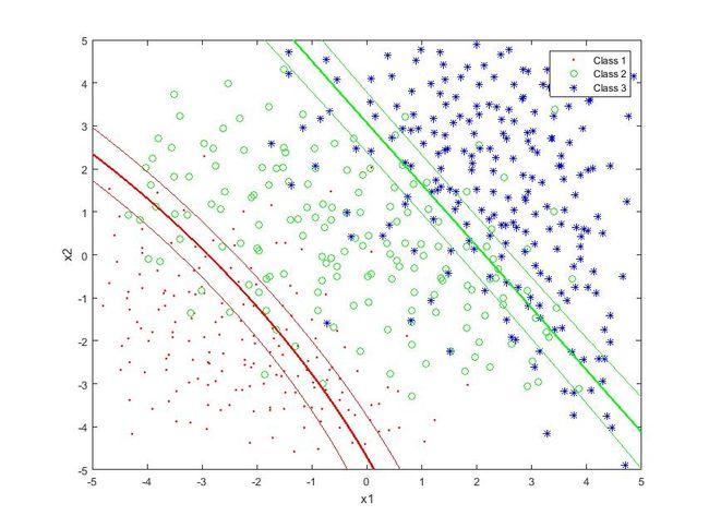
color = {'r.','go','b*','r.','go','b*'};
for i=1:max(y)
plot(X(y==i,1),X(y==i,2), color{i});
hold on
end
% include legend
% legend('Class 1', 'Class 2', 'Class 3','Location','NorthOutside', ...
% 'Orientation', 'horizontal');
legend('Class 1', 'Class 2', 'Class 3');
set(gca,'ydir','normal');
hold on
for k = 1:max(y)-1
decisionmapk = reshape(d(:,k), image_size);
contour(x1,x2, decisionmapk, [contour_level(1) contour_level(1) ], color{k},'Fill','off');
contour(x1,x2, decisionmapk, [contour_level(2) contour_level(2) ], color{k},'Fill','off','LineWidth',2);
contour(x1,x2, decisionmapk, [contour_level(3) contour_level(3) ], color{k},'Fill','off');
% if k
这里执行的是chu wei的支持向量顺序回归机模型SVORIM