梯度下降(Greadient Descent with squared error)
Gradient Descent with Squared Errors
We want to find the weights for our neural networks. Let's start by thinking about the goal. The network needs to make predictions as close as possible to the real values. To measure this, we use a metric of how wrong the predictions are, the error. A common metric is the sum of the squared errors (SSE):
![]()
where y_hat is the prediction and y is the true value, and you take the sum over all output units j and another sum over all data points μ. This might seem like a really complicated equation at first, but it's fairly simple once you understand the symbols and can say what's going on in words.
First, the inside sum over j. This variable j represents the output units of the network. So this inside sum is saying for each output unit, find the difference between the true value y and the predicted value from the network y_hat, then square the difference, then sum up all those squares.
Then the other sum over μ is a sum over all the data points. So, for each data point you calculate the inner sum of the squared differences for each output unit. Then you sum up those squared differences for each data point. That gives you the overall error for all the output predictions for all the data points.
The SSE is a good choice for a few reasons. The square ensures the error is always positive and larger errors are penalized more than smaller errors. Also, it makes the math nice, always a plus.
Remember that the output of a neural network, the prediction, depends on the weights

and accordingly the error depends on the weights
![E=\frac{1}{2} \sum_{u} \sum_{j}[y_{u}^{j}- \left [ f\left ( \sum_{i}w_{ij}x_{i}^{u} \right )\right ]^2](http://img.e-com-net.com/image/info8/62f78b2b19364555b3f6261a48fb233a.gif)
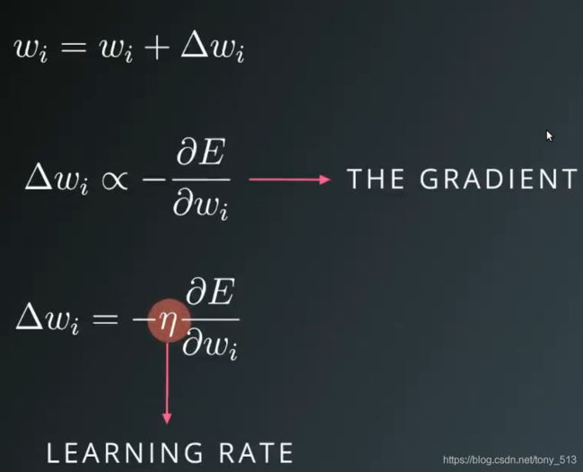
We want the network's prediction error to be as small as possible and the weights are the knobs we can use to make that happen. Our goal is to find weights w that minimize the squared error E. To do this with a neural network, typically you'd use gradient descent.
As Luis said, with gradient descent, we take multiple small steps towards our goal. In this case, we want to change the weights in steps that reduce the error. Continuing the analogy, the error is our mountain and we want to get to the bottom. Since the fastest way down a mountain is in the steepest direction, the steps taken should be in the direction that minimizes the error the most. We can find this direction by calculating the gradient of the squared error.
Gradient is another term for rate of change or slope. If you need to brush up on this concept, check out Khan Academy's great lectures on the topic.
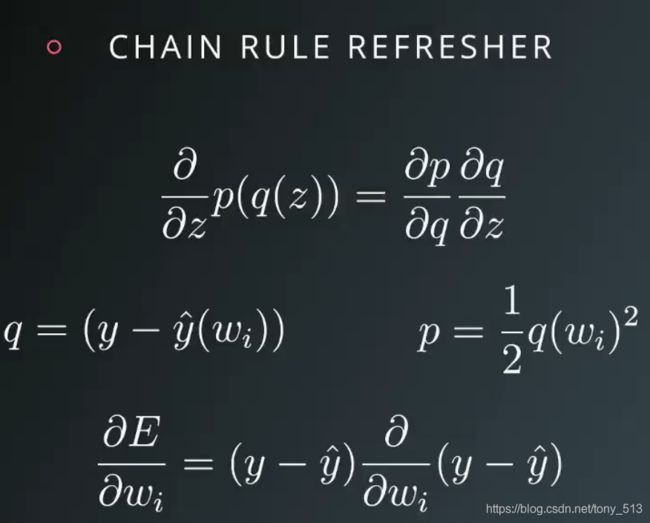
To calculate a rate of change, we turn to calculus, specifically derivatives. A derivative of a function f(x) gives you another function f′(x) that returns the slope of f(x) at point x. For example, consider f(x)=x^2. The derivative of x^2 is f′(x)=2x. So, at x=2, the slope is f′(2)=4. Plotting this out, it looks like:

The gradient is just a derivative generalized to functions with more than one variable. We can use calculus to find the gradient at any point in our error function, which depends on the input weights. You'll see how the gradient descent step is derived on the next page.
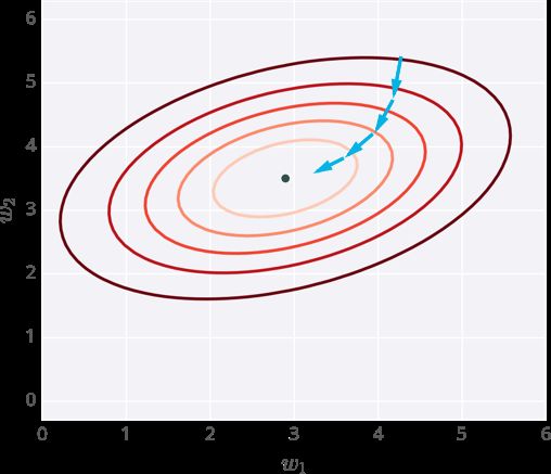
Below I've plotted an example of the error of a neural network with two inputs, and accordingly, two weights. You can read this like a topographical map where points on a contour line have the same error and darker contour lines correspond to larger errors.
At each step, you calculate the error and the gradient, then use those to determine how much to change each weight. Repeating this process will eventually find weights that are close to the minimum of the error function, the black dot in the middle.
 Gradient descent steps to the lowest errors
Caveats
Since the weights will just go wherever the gradient takes them, they can end up where the error is low, but not the lowest. These spots are called local minima. If the weights are initialized with the wrong values, gradient descent could lead the weights into a local minimum, illustrated below.
 Gradient descent leading into a local minimum
数学理解

y: true value ; y hat : predicted value ; W: weight , X: input
1. The error bettewn true vaule y and predicted value y hat ![]()
2. In order to get the positive error, we add a square sign to the function ![]() , The reason why not use absolute value is because square can penalize the outlilers more then small values.
, The reason why not use absolute value is because square can penalize the outlilers more then small values.
3. In order to geth the error of the whole dataset, we just need sum up the errors for each data record denoted by the sum over mu. ![]()
4. To clean up the math later, add a one half in front. ![]()
5. Remerbered that y hat is the linear combination of the weights inputs