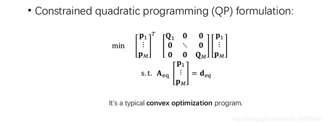
minimum snap轨迹规划 用二次规划QP求最优解
Minimum Snap 轨迹生成
一 解析解
算法思想:
1.给定起点 终点 经过点;
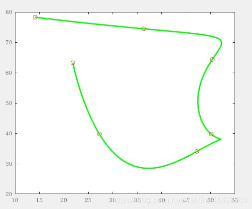
2.将所有点通过多项式连接,如图1;
3.起点终点(pvaj)限制;经过点(p)限制;
4.每一个segment多项式都不同,也就是每个segment的系数都是不同的,并不是用一条多项式将所有点相连,如图2所示,但是多项式的n_order相等;n_order=2×d_order-1;d_order表示优化目标的阶数;在此对snap进行优化,所以d_order=4;
5.这里采用分段计时,每个segment都有一个时间段T,如图3;


算法过程:
算法的过程难点就是再求解QP问题时,对QP二次型及限制条件的建立,也就是对QP中一些矩阵的建立
1.如图中4所示,Q矩阵为对称矩阵,Q中包含多个矩阵,每个小矩阵是每段多项式的的系数,有多少segmentQ就包含多少个Q_j;其中p为要求解优化的变量,p代表每个segment的系数,例如第一段的系数为p10,p11,…,p16;T为每个segment的时间;
2.手推一遍公式,Q的建立就很清楚了;
3.多项式的导数限制即为起点终点的pvaj,经过点的p;如图5
4.在建立矩阵时,因为Aj要与P相乘,前面说过p是所有多项式系数的一个组合,即p=(p10,p11…p16,p22…p26,…),所以在建立Aj矩阵时,注意Aj中元素的位置,使得A与P相乘时对应自己的系数p。得到Aeq_start,beq_start,Aeq_end,beq_end,Aeq_wp,beq_wp;
5.连续性约束即为前一段segment的终点与后一段segment的起点p是相等的;
6.这里就是把前一段seg的t=T带入多项式等于后面seg将t=0带入;这里就是0阶微分;
7.建立矩阵时前面的为+,后面的为-,与p相乘时=0;得到Aeq_con,beq_con
8.Aeq = [Aeq_start; Aeq_end; Aeq_wp; Aeq_con];
beq = [beq_start; beq_end; beq_wp; beq_con];
9. 通过求解器得到最优的系数poly_coef:poly_coef = quadprog(Q,f,[],[],Aeq, beq);因为p包含所有segment的系数p,所以还要将p分开,得到一组组的p系数p0 p1…p6;通过flipud将系数反转一下,得到从最高到最低的系数,再通过画图将曲线画出来
10. x和y都是关于t的多项式,所以将想x y分开求得到x关于t y关于t的多项式


MATLAB实现代码
主函数 hw1_1.m
clc;clear;close all;
path = ginput() * 100.0;

n_order       = 7;% order of poly
n_seg         = size(path,1)-1;% segment number
n_poly_perseg = (n_order+1); % coef number of perseg

ts = zeros(n_seg, 1);
% calculate time distribution in proportion to distance between 2 points
% dist     = zeros(n_seg, 1);
% dist_sum = 0;
% T        = 25;
% t_sum    = 0;
%
% for i = 1:n_seg
%     dist(i) = sqrt((path(i+1, 1)-path(i, 1))^2 + (path(i+1, 2) - path(i, 2))^2);
%     dist_sum = dist_sum+dist(i);
% end
% for i = 1:n_seg-1
%     ts(i) = dist(i)/dist_sum*T;
%     t_sum = t_sum+ts(i);
% end
% ts(n_seg) = T - t_sum;

% or you can simply set all time distribution as 1
for i = 1:n_seg
    ts(i) = 1.0;
end
testp = path(:,1);%path 的第一列
poly_coef_x = MinimumSnapQPSolver(path(:, 1), ts, n_seg, n_order);
poly_coef_y = MinimumSnapQPSolver(path(:, 2), ts, n_seg, n_order);


% display the trajectory
X_n = [];
Y_n = [];
k = 1;
tstep = 0.01;
for i=0:n_seg-1
    %#####################################################
    % STEP 3: get the coefficients of i-th segment of both x-axis
    % and y-axis
    start_idx = n_poly_perseg * i;
    Pxi = poly_coef_x(start_idx + 1 : start_idx + n_poly_perseg,1);
    Pxi = flipud(Pxi);
    Pyi = poly_coef_y(start_idx + 1 : start_idx + n_poly_perseg,1);
    Pyi = flipud(Pyi);
    for t = 0:tstep:ts(i+1)
        X_n(k)  = polyval(Pxi, t);
        Y_n(k)  = polyval(Pyi, t);
        k = k + 1;
    end
end

plot(X_n, Y_n , 'Color', [0 1.0 0], 'LineWidth', 2);
hold on
scatter(path(1:size(path, 1), 1), path(1:size(path, 1), 2));

function poly_coef = MinimumSnapQPSolver(waypoints, ts, n_seg, n_order)
    start_cond = [waypoints(1), 0, 0, 0];
    end_cond   = [waypoints(end), 0, 0, 0];
    %#####################################################
    % STEP 1: compute Q of p'Qp
    Q = getQ(n_seg, n_order, ts);
    %#####################################################
    % STEP 2: compute Aeq and beq
    [Aeq, beq] = getAbeq(n_seg, n_order, waypoints, ts, start_cond, end_cond);
    f = zeros(size(Q,1),1);
    poly_coef = quadprog(Q,f,[],[],Aeq, beq);
end
建立Q对称矩阵
function Q = getQ(n_seg, n_order, ts)
    Q = [];
    for j = 0:n_seg-1
        Q_j = zeros(8,8);
        %#####################################################
        % STEP 1.1: calculate Q_k of the k-th segment
        %%%%%%%%%%%%%%%%%%%%%%%%%%%%%%%%%%%%%%%%%%%%%%%%%%%%%%
        for i=4:n_order
            for l=4:n_order
                L = factorial(l)/factorial(l-4);
                I = factorial(i)/factorial(i-4);
                Q_j(i+1,l+1) = L*I/(i+l-7);
            end
        end
        Q = blkdiag(Q, Q_j);
    end
end
建立Aeq矩阵和beq
function [Aeq beq]= getAbeq(n_seg, n_order, waypoints, ts, start_cond, end_cond)
    n_all_poly = n_seg*(n_order+1);
    %#####################################################
    % p,v,a,j constraint in start,
    Aeq_start = zeros(4, n_all_poly);
    beq_start = zeros(4, 1);
    % STEP 2.1: write expression of Aeq_start and beq_start
    for k= 0:3
        Aeq_start(k+1,k+1) = factorial(k);
    end
    beq_start = start_cond';
    %#####################################################
    % p,v,a constraint in end
    Aeq_end = zeros(4, n_all_poly);
    beq_end = zeros(4, 1);
    % STEP 2.2: write expression of Aeq_end and beq_end
    start_idx_2 = (n_order + 1)*(n_seg - 1);
    for k=0 : 3
        for i=k : 7
            Aeq_end(k+1,start_idx_2 + 1 + i ) = factorial(i)/factorial(i-k)*ts(n_seg)^(i-k);
        end
    end
    beq_end = end_cond';

    %#####################################################
    % position constrain in all middle waypoints
    Aeq_wp = zeros(n_seg-1,n_all_poly);
    beq_wp = zeros(n_seg-1,1);
    for i=0:n_seg-2
        start_idx_2 = (n_order + 1)*(i+1);
        Aeq_wp(i+1,start_idx_2+1) = 1;
        beq_wp(i+1,1) = waypoints(i+2);
    end

    Aeq_con = zeros((n_seg-1)*4, n_all_poly);
    beq_con = zeros((n_seg-1)*4, 1);
    for k=0:3
        for j=0:n_seg-2
            for i = k:7
                start_idx_1 = (n_seg-1)*k;
                start_idx_2 = (n_order+1)*j;
                Aeq_con(start_idx_1 + j + 1,start_idx_2 + i+1)=...
                    factorial(i)/factorial(i-k)*ts(j+1)^(i-k);
                if(i == k)
                    Aeq_con(start_idx_1+j+1,start_idx_2+(n_order+1)+i+1) = ...
                                                            -factorial(i);
                end
            end
        end
    end


    %#####################################################
    % combine all components to form Aeq and beq
    Aeq = [Aeq_start; Aeq_end; Aeq_wp; Aeq_con];
    beq = [beq_start; beq_end; beq_wp; beq_con];
end
仿真结果
二 闭式解 close-form
解析解只能得出结果,别人只能利用这个结果
闭式解可以得到解的解析式,别人可以利用解析式求解
在轨迹生成中,解析解中的限制条件没有物理意义,而且数值会在高次产生不稳定性,所以要把对系数(无物理意义)的优化变为对va的优化。
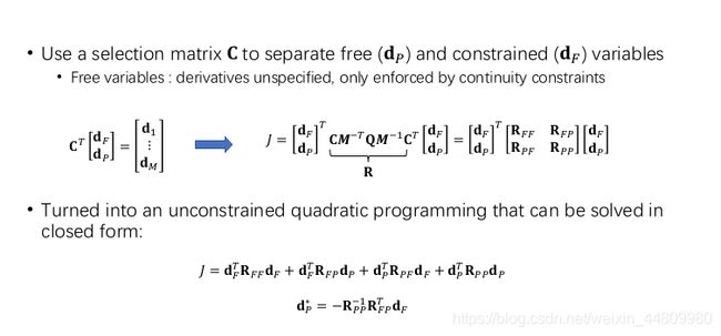
主要思想
通过映射矩阵M将P与限制条件d相连产生关系。d又可以通过选择矩阵Ct把d中的fix条件和free条件分开为dF dP.所以P就可以换成与条件有关的矩阵,通过qp得到闭式解。


算法过程
过程与前面解析解过程一样,只是建立的矩阵不同。
代码
主函数hw1_2
clc;clear;close all;
path = ginput() * 100.0;

n_order = 7;
n_seg = size(path, 1) - 1;
n_poly_perseg = n_order + 1;

ts = zeros(n_seg, 1);
% calculate time distribution based on distance between 2 points
dist = zeros(n_seg, 1);
dist_sum = 0;
T = 25;

t_sum = 0;
for i = 1:n_seg
    dist(i) = sqrt((path(i+1, 1) - path(i, 1))^2 + (path(i+1, 2) - path(i, 2))^2);
    dist_sum = dist_sum + dist(i);
end
for i = 1:n_seg-1
    ts(i) = dist(i) / dist_sum * T;
    t_sum = t_sum + ts(i);
end
ts(n_seg) = T - t_sum;
% or you can simply average the time
% for i = 1:n_seg
%     ts(i) = 1.0;
% end

poly_coef_x = MinimumSnapCloseformSolver(path(:, 1), ts, n_seg, n_order);
poly_coef_y = MinimumSnapCloseformSolver(path(:, 2), ts, n_seg, n_order);

X_n = [];
Y_n = [];
k = 1;
tstep = 0.01;
for i=0:n_seg-1
    %#####################################################
    % STEP 4: get the coefficients of i-th segment of both x-axis
    % and y-axis
    start_idx = n_poly_perseg* i;
    Pxi = poly_coef_x(start_idx+1:start_idx+n_poly_perseg,1);
    Pxi = flipud(Pxi);
    Pyi = poly_coef_y(start_idx+1:start_idx+n_poly_perseg,1);
    Pyi = flipud(Pyi);
    for t=0:tstep:ts(i+1)
        X_n(k)  = polyval(Pxi,t);
        Y_n(k)  = polyval(Pyi,t);
        k = k+1;
    end
end

plot(X_n, Y_n ,'Color',[0 1.0 0],'LineWidth',2);
hold on
scatter(path(1:size(path,1),1),path(1:size(path,1),2));

function poly_coef = MinimumSnapCloseformSolver(waypoints, ts, n_seg, n_order)
    start_cond = [waypoints(1), 0, 0, 0];
    end_cond =   [waypoints(end), 0, 0, 0];
    %#####################################################
    % you have already finished this function in hw1
    Q = getQ(n_seg, n_order, ts);
    %#####################################################
    % STEP 1: compute M
    M = getM(n_seg, n_order, ts);
    %#####################################################
    % STEP 2: compute Ct
    Ct = getCt(n_seg, n_order);
    C = Ct';
    invMt=inv(M)';
    R = C * inv(M)' * Q * inv(M) * Ct;
    R_cell = mat2cell(R, [n_seg+7 ,3*(n_seg-1)], [n_seg+7 ,3*(n_seg-1)]);%矩阵分块
    R_pp = R_cell{2, 2};
    R_fp = R_cell{1, 2};
    %#####################################################
    % STEP 3: compute dF
    dF = [start_cond'; waypoints(2:end-1); end_cond'];
    dP = -inv(R_pp) * R_fp' * dF;
    poly_coef = inv(M) * Ct * [dF;d
end
建立M矩阵 getM
function M = getM(n_seg, n_order, ts)
    M = [];
    d_order = 4;
    n_order = 7;
    for j = 1:n_seg
        M_k = [];
        %#####################################################
        % STEP 1.1: calculate M_k of the k-th segment
        %其实这里的M矩阵是和n_order和d_order有关的
        %矩阵规模为:2*d_order X (n_order+1);
        %对多项式求0 1 2 3 次导,将t=0 和 t=T带入,得到矩阵里面的数
        %%%%%%%%%%%%%%%%%%%%%%%%%%%%%%%%%%%%%%%%%%%%%%%%%%%%%%%
        for k=0:d_order-1
            M_k(k+1,k+1) = factorial(k);
            for i=k:n_order
                M_k(k+1+4,i+1)=factorial(i)/factorial(i-k)*ts(j)^(i-k);
            end
        end
        M = blkdiag(M, M_k);
    end
end
建立Ct矩阵 getCt
function Ct = getCt(n_seg, n_order)
    %#####################################################
    % STEP 2.1: finish the expression of Ct
    %%%%%%%%%%%%%%%%%%%%%%%%%%%%%%%%%%%%%%%%%%%%%%%%%%%%%%
    %ct for start point
    d_order = 4;
    Ct_start = zeros(d_order,d_order*(n_seg+1));
    Ct_start(:,1:d_order) = eye(d_order);


    %Ct for middle points
    %n_seg轨迹有n_seg -1 个waypoint,每个wp有2X4个条件所以:2*4*(n_seg-1)
    Ct_mid = zeros(2*d_order*(n_seg-1),d_order*(n_seg+1));
    %0:seg-2 为一共seg-1个点
    for j = 0:n_seg-2
        Cj = zeros(d_order,d_order*(n_seg+1));
        Cj (1,d_order+j+1) =1;
        start_idx_2 = 2*d_order+n_seg-1+3*j;%
        Cj(2:d_order,start_idx_2+1:start_idx_2+3) = eye(d_order-1);
        %截止到这行,实现的是wypoint的前一段t=T时刻的pvaj,
        %后面实现的是wypoint后一段t=0时刻的pvaj,
        %并将wypoint2Xd_order,8个条件放入一个矩阵中
        start_idx_1 = 2*d_order*j;
        Ct_mid(start_idx_1+1:start_idx_1+2*d_order,:) = [Cj;Cj];
        %因为条件pvaj相同,所以C的矩阵也和上一段t=T时刻的c一样。
    end
    %Ct for end point
    Ct_end = zeros(d_order,d_order*(n_seg+1));
    Ct_end(:,d_order+n_seg:2*d_order+n_seg-1) = eye(d_order);

    Ct=[Ct_start;Ct_mid;Ct_end];
end
仿真结果

代码细节问题
1.怎么建立M
M * Pj = dj
- d为限制条件,即[p v a j ]’;
- P为多项式系数,即[p0 p1 p2, p3 p4 p5,p6 p7]’;
- 所以根据d和p,不难建立出M;
2.怎么建立Ct
Ct * [dF dP]’ = [d1 …dm]’;
- Ct为选择矩阵 我们要建立的;
- dF为fix限制条件,即起点终点的 [p v a j],wypoint的 p;
- dP为free条件,即wapoint的[v a j];
- d1…dm为所有点的条件 p v a j
Ct 如下图所示:
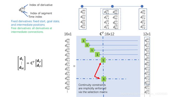
Ct可以分为三部分:
Ct = [ Ct_start Ct_wy Ct_end ]’
- 第一部分为与起始点有关的Ct_start;
- 第二部分为与wypoint有关的Ct_wy;
- 第三部分为与终点有关的Ct_end;