Kaggle playground 练习项目 New York City Taxi Trip Duration

       最近接触了一些机器学习知识，想在kaggle上找入门项目做做练手。于是选择了New York City Taxi Trip Duration这个预测出租车行驶时间的练习赛。

     训练集特征包括以下部分，目的是建立模型预测出租车每次行程的行驶时间。

    id - 每次旅行的唯一标识符
    vendor_id - 指示与旅行记录关联的提供者的代码
    pickup_datetime - 仪表启用的日期和时间
    dropoff_datetime - 仪表脱离的日期和时间
    passenger_count - 车辆中的乘客数量（驾驶员输入值）
    pickup_longitude - 仪表所用的经度
    pickup_latitude - 仪表所处的纬度
    dropoff_longitude - 仪表脱离的经度
    dropoff_latitude - 仪表脱离的纬度
    store_and_fwd_flag - 该标志指示在发送给供应商之前是否将行程记录保存在车辆存储器中，因为车辆没有连接到服务器

                                       Y =存储和转发; N =不是商店和前瞻旅行
    trip_duration - 行程的持续时间，以秒为单位

    评分根据为RMSE（均方根误差）。

 

        以下是一个使用随机森林预测的简单初步模型。

 

# -*- coding: utf-8 -*-

import pandas as pd

train = pd.read_csv("train.csv", header=0)
test = pd.read_csv("test.csv", header=0)

# 查看数据的字段信息, dropoff_datetime,id可以去掉
# print(train.columns)
# print(test.columns)

# 查看数据是否有缺失
# print(train.info())
# print(test.info())

# 选取特征值
X_train = train.drop(['dropoff_datetime', 'trip_duration', 'id'], axis=1)
y_train = train['trip_duration']
X_test = test.drop(['id'], axis=1)

# print(X_train.shape)
# print(X_test.shape)
# print(y_train.head())

# 特征值处理
X_train['month'] = pd.DatetimeIndex(X_train.pickup_datetime).month
X_train['day'] = pd.DatetimeIndex(X_train.pickup_datetime).dayofweek
X_train['hour'] = pd.DatetimeIndex(X_train.pickup_datetime).hour
X_train['store_and_fwd_flag'].replace('Y', 1, inplace=True)
X_train['store_and_fwd_flag'].replace('N', 0, inplace=True)
X_train = X_train.drop(['pickup_datetime'], axis=1)

X_test['month'] = pd.DatetimeIndex(X_test.pickup_datetime).month
X_test['day'] = pd.DatetimeIndex(X_test.pickup_datetime).dayofweek
X_test['hour'] = pd.DatetimeIndex(X_test.pickup_datetime).hour
X_test['store_and_fwd_flag'].replace('Y', 1, inplace=True)
X_test['store_and_fwd_flag'].replace('N', 0, inplace=True)
X_test = X_test.drop(['pickup_datetime'], axis=1)
# print(X_test['store_and_fwd_flag'].value_counts())
# print(X_train.head())
# print(X_test.head())
# print(X_train.shape)
# print(X_test.shape)

# 使用RandomForestRegressor进行回归预测
from sklearn.ensemble import RandomForestRegressor
rfr = RandomForestRegressor()
rfr.fit(X_train, y_train)
rfr_y_predict = rfr.predict(X_test)


# 输出结果
gbr_submission = pd.DataFrame({'id': test['id'], 'trip_duration': rfr_y_predict})
gbr_submission.to_csv('rfr_submission.csv', index=False)

最终分数为0.55480，还有很大的提升空间。

下面是一个进行了比较完善的特征工程，并且使用了模型融合的解法。

 导入各种计算包

import pandas as pd
pd.set_option('display.max_columns', None)
import numpy as np
import tensorflow as tf

from sklearn.ensemble import RandomForestRegressor as RFR
import lightgbm as lgb
from catboost import CatBoostRegressor

from collections import namedtuple
from pandas.tseries.holiday import USFederalHolidayCalendar
from pandas.tseries.offsets import CustomBusinessDay

import time
import operator
import haversine
from sklearn.cluster import KMeans
from sklearn.decomposition import PCA
from sklearn.model_selection import train_test_split
from sklearn.metrics import mean_squared_error
from datetime import timedelta
import seaborn as sns
import matplotlib.pyplot as plt
%matplotlib inline  

读入数据

train = pd.read_csv("train.csv")
test = pd.read_csv("test.csv")

确定没有重复和错误数据

print(train.duplicated().sum())
print(train.id.duplicated().sum())
print(test.id.duplicated().sum())

sum(train.dropoff_datetime < train.pickup_datetime)

数据清洗

train = train.drop('dropoff_datetime',1)
train.trip_duration.describe()

# Values are in minutes
print(np.percentile(train.trip_duration, 99)/60)
print(np.percentile(train.trip_duration, 99.5)/60)
print(np.percentile(train.trip_duration, 99.6)/60)
print(np.percentile(train.trip_duration, 99.8)/60)
print(np.percentile(train.trip_duration, 99.85)/60)
print(np.percentile(train.trip_duration, 99.9)/60)
print(np.percentile(train.trip_duration, 99.99)/60)
print(np.percentile(train.trip_duration, 99.999)/60)
print(np.percentile(train.trip_duration, 99.9999)/60)
print(train.trip_duration.max() / 60)

通过上面的操作可以看见，有些旅程记录耗费时间太多，应该作为离群点删去，否则会对模型预测造成影响。

# Check how many trips remain with each limit
print(len(train[train.trip_duration <= np.percentile(train.trip_duration, 99.9)]))
print(len(train[train.trip_duration <= np.percentile(train.trip_duration, 99.99)]))
print(len(train[train.trip_duration <= np.percentile(train.trip_duration, 99.999)]))

# Remove outliers
train = train[train.trip_duration <= np.percentile(train.trip_duration, 99.999)]

对训练集作图，查找离群点。

# Plot locations - look for outliers
n = 100000 # number of data points to display

f, (ax1, ax2) = plt.subplots(1, 2, sharey=True, figsize=(10, 5))
ax1.scatter(train.pickup_longitude[:n], 
            train.pickup_latitude[:n],
            alpha = 0.1)
ax1.set_title('Pickup')
ax2.scatter(train.dropoff_longitude[:n], 
            train.dropoff_latitude[:n],
            alpha = 0.1)
ax2.set_title('Dropoff')

图像如下所示

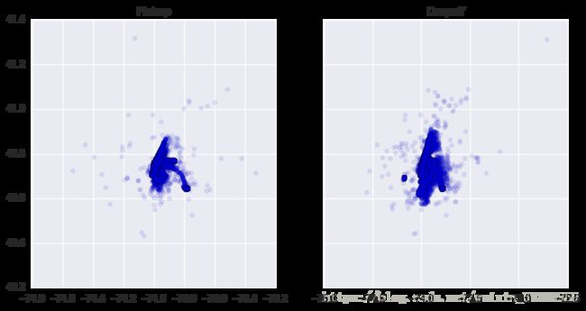
从图像上看还算相对比较集中，但是我们还是要对数据进行一定的修剪，从而提高模型训练效果。

# The values are not too wild, but we'll trim them back a little to be conservative
print(train.pickup_latitude.max())
print(train.pickup_latitude.min())
print(train.pickup_longitude.max())
print(train.pickup_longitude.min())
print()
print(train.dropoff_latitude.max())
print(train.dropoff_latitude.min())
print(train.dropoff_longitude.max())
print(train.dropoff_longitude.min())


# Find limits of location
max_value = 99.999
min_value = 0.001

max_pickup_lat = np.percentile(train.pickup_latitude, max_value)
min_pickup_lat = np.percentile(train.pickup_latitude, min_value)
max_pickup_long = np.percentile(train.pickup_longitude, max_value)
min_pickup_long = np.percentile(train.pickup_longitude, min_value)

max_dropoff_lat = np.percentile(train.dropoff_latitude, max_value)
min_dropoff_lat = np.percentile(train.dropoff_latitude, min_value)
max_dropoff_long = np.percentile(train.dropoff_longitude, max_value)
min_dropoff_long = np.percentile(train.dropoff_longitude, min_value)


# Remove extreme values
train = train[(train.pickup_latitude <= max_pickup_lat) & (train.pickup_latitude >= min_pickup_lat)]
train = train[(train.pickup_longitude <= max_pickup_long) & (train.pickup_longitude >= min_pickup_long)]

train = train[(train.dropoff_latitude <= max_dropoff_lat) & (train.dropoff_latitude >= min_dropoff_lat)]
train = train[(train.dropoff_longitude <= max_dropoff_long) & (train.dropoff_longitude >= min_dropoff_long)]

重新绘图来观察处理离群点前后的变化。

# Replot to see the differences - minimal, but there is some change
f, (ax1, ax2) = plt.subplots(1, 2, sharey=True, figsize=(10, 5))
ax1.scatter(train.pickup_longitude[:n], 
            train.pickup_latitude[:n],
            alpha = 0.1)
ax1.set_title('Pickup')
ax2.scatter(train.dropoff_longitude[:n], 
            train.dropoff_latitude[:n],
            alpha = 0.1)
ax2.set_title('Dropoff')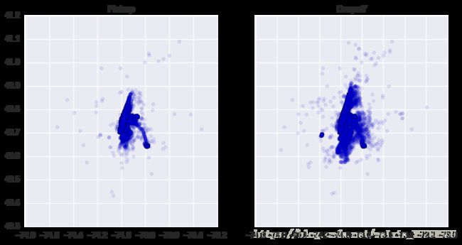

 

      

   可以看到几个离群点被删去，数据变得更加集中。

特征工程

    将训练集和测试集合并在一起，方便进行特征工程。

# Concatenate the datasets for feature engineering
df = pd.concat([train,test])

df.shape

   查看有无缺失值。

# Check for null values
# trip_duration nulls to due to them not being present in the test set
df.isnull().sum()

dropoff_latitude           0
dropoff_longitude          0
id                         0
passenger_count            0
pickup_datetime            0
pickup_latitude            0
pickup_longitude           0
store_and_fwd_flag         0
trip_duration         625134
vendor_id                  0
dtype: int64

 可以看出数据没有缺失值。

 将csv中String类型的格式转为时间格式。

df.vendor_id.value_counts()

print(train.pickup_datetime.max())
print(train.pickup_datetime.min())
print()
print(test.pickup_datetime.max())
print(test.pickup_datetime.min())
print()
print(df.pickup_datetime.max())
print(df.pickup_datetime.min())

# Convert to datetime
df.pickup_datetime = pd.to_datetime(df.pickup_datetime)

将接客时间点转为用分钟表示。

# Calculate what minute in a day the pickup is at
df['pickup_minute_of_the_day'] = df.pickup_datetime.dt.hour*60 + df.pickup_datetime.dt.minute

将接客时间点使用K-均值算法聚类为24个时间段，对应一天24小时，考虑到上下班高峰期，每个时间段的样本数量应该有明显的不同。

# Rather than use the standard 24 hours, group the trips into 24 groups that are sorted by KMeans
# This should help 'rush-hour' rides to be in the same groups
kmeans_pickup_time = KMeans(n_clusters=24, random_state=2).fit(df.pickup_minute_of_the_day[:500000].values.reshape(-1,1))

df['kmeans_pickup_time'] = kmeans_pickup_time.predict(df.pickup_minute_of_the_day.values.reshape(-1,1))

将使用K-均值聚类分出的时间区间和标准的一天24小时进行对比，可以发现明显的高峰期时段。

# Compare the distribution of kmeans_pickup_time and the standard 24 hour breakdown
n = 50000 # number of data points to plot
f, (ax1, ax2) = plt.subplots(2, 1, sharex=True, figsize=(10, 5))

ax1.scatter(x = df.pickup_minute_of_the_day[:n]/60, 
            y = np.random.uniform(0,1, n), 
            cmap = 'Set1',
            c = df.kmeans_pickup_time[:n])
ax1.set_title('KMeans Pickup Time')

ax2.scatter(x = df.pickup_minute_of_the_day[:n]/60, 
            y = np.random.uniform(0,1, n), 
            cmap = 'Set1',
            c = df.pickup_datetime.dt.hour[:n])
ax2.set_title('Pickup Hour')

   根据是否是周末、节假日和工作日等创造新特征。

# Load a list of holidays in the US
calendar = USFederalHolidayCalendar()
holidays = calendar.holidays()

# Load business days
us_bd = CustomBusinessDay(calendar = USFederalHolidayCalendar())
# Set business_days equal to the work days in our date range.
business_days = pd.DatetimeIndex(start = df.pickup_datetime.min(), 
                                 end = df.pickup_datetime.max(), 
                                 freq = us_bd)
business_days = pd.to_datetime(business_days).date

# Create features relating to time
df['pickup_month'] = df.pickup_datetime.dt.month
df['pickup_weekday'] = df.pickup_datetime.dt.weekday
df['pickup_is_weekend'] = df.pickup_weekday.map(lambda x: 1 if x >= 5 else 0)
df['pickup_holiday'] = pd.to_datetime(df.pickup_datetime.dt.date).isin(holidays)
df['pickup_holiday'] = df.pickup_holiday.map(lambda x: 1 if x == True else 0)

# If day is before or after a holiday
df['pickup_near_holiday'] = (pd.to_datetime(df.pickup_datetime.dt.date).isin(holidays + timedelta(days=1)) |
                             pd.to_datetime(df.pickup_datetime.dt.date).isin(holidays - timedelta(days=1)))
df['pickup_near_holiday'] = df.pickup_near_holiday.map(lambda x: 1 if x == True else 0)
df['pickup_businessday'] = pd.to_datetime(df.pickup_datetime.dt.date).isin(business_days)
df['pickup_businessday'] = df.pickup_businessday.map(lambda x: 1 if x == True else 0)

创建week_delta新特征，将接客时间换算成每一周中的具体时间。

# Calculates what minute of the week it is
df['week_delta'] = (df.pickup_weekday + ((df.pickup_datetime.dt.hour + 
                                              (df.pickup_datetime.dt.minute / 60.0)) / 24.0))

根据接客时间的月份、日期、是否是周末和节假日等进行分组，并添加到数据集中。

# Determines number of rides that occur during each specific time
# Should help to determine traffic
ride_counts = df.groupby(['pickup_month', 'pickup_weekday','pickup_holiday','pickup_near_holiday',
            'pickup_businessday','kmeans_pickup_time']).size()
ride_counts = pd.DataFrame(ride_counts).reset_index()
ride_counts['ride_counts'] = ride_counts[0]
ride_counts = ride_counts.drop(0,1)

# Add `ride_counts` to dataframe
df = df.merge(ride_counts, on=['pickup_month',
                          'pickup_weekday',
                          'pickup_holiday',
                          'pickup_near_holiday',
                          'pickup_businessday',
                          'kmeans_pickup_time'], how='left')

经过上述处理后，已经不再需要pickup_datetime这个特征。

# Dont' need this feature any more
df = df.drop('pickup_datetime', 1)

将接客和下客的地点经度和纬度使用K均值算法分成15个聚类。

kmeans_pickup = KMeans(n_clusters=15, random_state=2).fit(df[['pickup_latitude','pickup_longitude']][:500000])
kmeans_dropoff = KMeans(n_clusters=15, random_state=2).fit(df[['dropoff_latitude','dropoff_longitude']][:500000])

df['kmeans_pickup'] = kmeans_pickup.predict(df[['pickup_latitude','pickup_longitude']])
df['kmeans_dropoff'] = kmeans_dropoff.predict(df[['dropoff_latitude','dropoff_longitude']])

将这15个聚类画出来。

# Plot these 15 groups

n = 100000 # Number of data points to plot
f, (ax1, ax2) = plt.subplots(1, 2, sharey=True, figsize=(10, 5))
ax1.scatter(df.pickup_longitude[:n], 
            df.pickup_latitude[:n],
            cmap = 'viridis',
            c = df.kmeans_pickup[:n])
ax1.set_title('Pickup')
ax2.scatter(df.dropoff_longitude[:n], 
            df.dropoff_latitude[:n],
            cmap = 'viridis',
            c = df.kmeans_dropoff[:n])
ax2.set_title('Dropoff')

    使用PCA算法将接客点和下客点的经纬度合并成一个特征。

# Reduce pickup and dropoff locations to one value
pca = PCA(n_components=1)
df['pickup_pca'] = pca.fit_transform(df[['pickup_latitude','pickup_longitude']])
df['dropoff_pca'] = pca.fit_transform(df[['dropoff_latitude','dropoff_longitude']])

创建距离特征，包括平面距离、半径距离、曼哈顿距离以及它们的对数。

# Create distance features
df['distance'] = np.sqrt(np.power(df['dropoff_longitude'] - df['pickup_longitude'], 2) + 
                         np.power(df['dropoff_latitude'] - df['pickup_latitude'], 2))
df['haversine_distance'] = df.apply(lambda r: haversine.haversine((r['pickup_latitude'],r['pickup_longitude']),
                                                                  (r['dropoff_latitude'], r['dropoff_longitude'])), 
                           axis=1)
df['manhattan_distance'] = (abs(df.dropoff_longitude - df.pickup_longitude) +
                            abs(df.dropoff_latitude - df.pickup_latitude))
df['log_distance'] = np.log(df['distance'] + 1)
df['log_haversine_distance'] = np.log(df['haversine_distance'] + 1)
df['log_manhattan_distance'] = np.log(df.manhattan_distance + 1)

定义一个函数，用来计算用弧度表示的方向。同时创建方向特征。

def calculate_bearing(pickup_lat, pickup_long, dropoff_lat, dropoff_long):
    '''Calculate the direction of travel in degrees'''
    pickup_lat_rads = np.radians(pickup_lat)
    pickup_long_rads = np.radians(pickup_long)
    dropoff_lat_rads = np.radians(dropoff_lat)
    dropoff_long_rads = np.radians(dropoff_long)
    long_delta_rads = np.radians(dropoff_long_rads - pickup_long_rads)
    
    y = np.sin(long_delta_rads) * np.cos(dropoff_lat_rads)
    x = (np.cos(pickup_lat_rads) * 
         np.sin(dropoff_lat_rads) - 
         np.sin(pickup_lat_rads) * 
         np.cos(dropoff_lat_rads) * 
         np.cos(long_delta_rads))
    
    return np.degrees(np.arctan2(y, x))

df['bearing'] = calculate_bearing(df.pickup_latitude,
                                  df.pickup_longitude,
                                  df.dropoff_latitude,
                                  df.dropoff_longitude)

对乘客数量进行统计，同时创建四个新特征，分别对应四个区间的乘客数量。

df.passenger_count.value_counts()

# Group passenger_count by type of group
df['no_passengers'] = df.passenger_count.map(lambda x: 1 if x == 0 else 0)
df['one_passenger'] = df.passenger_count.map(lambda x: 1 if x == 1 else 0)
df['few_passengers'] = df.passenger_count.map(lambda x: 1 if x > 1 and x <= 4 else 0)
df['many_passengers'] = df.passenger_count.map(lambda x: 1 if x >= 5 else 0)

将定性特征转化为定量特征，以及对上述K均值算法分出的区间和月份，日期进行one-hot处理。

df.store_and_fwd_flag = df.store_and_fwd_flag.map(lambda x: 1 if x == 'Y' else 0)


# Create dummy features for these features, then drop these features
dummies = ['kmeans_pickup_time','pickup_month','pickup_weekday','kmeans_pickup','kmeans_dropoff']
for feature in dummies:
    dummy_features = pd.get_dummies(df[feature], prefix=feature)
    for dummy in dummy_features:
        df[dummy] = dummy_features[dummy]
    df = df.drop([feature], 1)

丢弃id特征。

# Don't need this feature any more
df = df.drop(['id'],1)

对除了trip_duration以外的特征进行mean normalization处理，提高模型拟合效率。

# Transform each feature to have a mean of 0 and standard deviation of 1
# Help to train the neural network
for feature in df:
    if feature == 'trip_duration':
        continue
    mean, std = df[feature].mean(), df[feature].std()
    df.loc[:, feature] = (df[feature] - mean)/std

将数据集返回到训练集和测试集状态，并从训练集中提取出交叉验证集。

# Return data into a training and testing set
trainFinal = df[:-len(test)]
testFinal = df[-len(test):]

# Give trip_duration its own dataframe
# Drop it from the other dataframes
yFinal = pd.DataFrame(trainFinal.trip_duration)
trainFinal = trainFinal.drop('trip_duration',1)
testFinal = testFinal.drop('trip_duration',1)

# Sort data into training and testing sets
x_trainFinal, x_testFinal, y_trainFinal, y_testFinal = train_test_split(trainFinal, 
                                                                    np.log(yFinal+1), 
                                                                        test_size=0.15, 
                                                                        random_state=2)

x_train, x_test, y_train, y_test = train_test_split(x_trainFinal, 
                                                    y_trainFinal, 
                                                    test_size=0.15,
                                                    random_state=2)

建模和训练

     原作者使用了神经网络训练，此处先按下不表，先关注后边用随机森林和xgboost训练的部分。

随机森林回归

  

# Create an empty dataframe to contain all of the inputs for each iteration of the model
results_rfr = pd.DataFrame(columns=["RMSE",
                                    "n_estimators", 
                                    "max_depth", 
                                    "min_samples_split"])

for i in range(num_iterations):
    # Use random search to choose the inputs' values
    n_estimators = np.random.randint(10,20)
    max_depth = np.random.randint(6,12)
    min_samples_split = np.random.randint(2,50)

    rfr = RFR(n_estimators = n_estimators,
          max_depth = max_depth,
          min_samples_split = min_samples_split,
          verbose = 2,
          random_state = 2)
    
    rfr = rfr.fit(x_train, y_train.values)

    y_preds_rfr = rfr.predict(x_testFinal)
    RMSE_rfr = np.sqrt(mean_squared_error(y_testFinal, y_preds_rfr))
    print("RMSE for iteration #{} is {}.".format(i+1, RMSE_rfr))
    print("NE={}, MD={}, MSS={}".format(n_estimators,
                                        max_depth,
                                        min_samples_split))
    print()
    initial_preds[RMSE_rfr] = y_preds_rfr
    testFinal_preds_rfr = rfr.predict(testFinal)
    final_preds[RMSE_rfr] = [testFinal_preds_rfr]
    
    # Create a dataframe with the values above
    new_row = pd.DataFrame([[RMSE_rfr,
                             n_estimators, 
                             max_depth, 
                             min_samples_split]],
                     columns = ["RMSE",
                                "n_estimators", 
                                "max_depth", 
                                "min_samples_split"])
    
    # Append the dataframe as a new row in results_df
    results_rfr = results_rfr.append(new_row, ignore_index=True)

训练结果如下

 

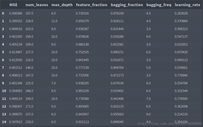
用同样的方法使用LightGBM Regressor训练和调参

# Create an empty dataframe to contain all of the inputs for each iteration of the model
results_lgb = pd.DataFrame(columns=["RMSE",
                                    "num_leaves", 
                                    "max_depth", 
                                    "feature_fraction",
                                    "bagging_fraction",
                                    "bagging_freq",
                                    "learning_rate"])

for i in range(num_iterations):
    
    num_leaves = np.random.randint(100,250)
    max_depth = np.random.randint(6,12)
    feature_fraction = np.random.uniform(0.7,1)
    bagging_fraction = np.random.uniform(0.8,1)
    bagging_freq = np.random.randint(3,10)
    learning_rate = np.random.uniform(0.2,1)
    n_estimators = 100
    early_stopping_rounds = 5

    gbm = lgb.LGBMRegressor(objective = 'regression',
                            boosting_type = 'gbdt',
                            num_leaves = num_leaves,
                            max_depth = max_depth,
                            feature_fraction = feature_fraction,
                            bagging_fraction = bagging_fraction,
                            bagging_freq = bagging_freq,
                            learning_rate = learning_rate,
                            n_estimators = n_estimators)
    
    gbm.fit(x_train.values, y_train.values.ravel(),
            eval_set = [(x_test.values, y_test.values.ravel())],
            eval_metric = 'rmse',
            early_stopping_rounds = early_stopping_rounds)

    y_preds_gbm = gbm.predict(x_testFinal, num_iteration = gbm.best_iteration)
    RMSE_gbm = np.sqrt(mean_squared_error(y_testFinal, y_preds_gbm))
    print("RMSE for iteration #{} is {}.".format(i+1, RMSE_gbm))
    print("NL={}, MD={}, FF={}, BF={}, BQ={}, LR={}, NE={}, ESR={}".format(num_leaves,
                                                                           max_depth,
                                                                           feature_fraction,
                                                                           bagging_fraction,
                                                                           bagging_freq,
                                                                           learning_rate,
                                                                           n_estimators,
                                                                           early_stopping_rounds))
    print()
    initial_preds[RMSE_gbm] = y_preds_gbm
    testFinal_preds_gbm = gbm.predict(testFinal, num_iteration = gbm.best_iteration)
    final_preds[RMSE_gbm] = [testFinal_preds_gbm]
    
    # Create a dataframe with the values above
    new_row = pd.DataFrame([[RMSE_gbm,
                             num_leaves, 
                             max_depth, 
                             feature_fraction,
                             bagging_fraction,
                             bagging_freq,
                             learning_rate]],
                     columns = ["RMSE",
                                "num_leaves", 
                                "max_depth", 
                                "feature_fraction",
                                "bagging_fraction",
                                "bagging_freq",
                                "learning_rate"])
    
    # Append the dataframe as a new row in results_df
    results_lgb = results_lgb.append(new_row, ignore_index=True)

结果如下：

CatBoostRegressor

# Create an empty dataframe to contain all of the inputs for each iteration of the model
results_cbr = pd.DataFrame(columns=["RMSE",
                                    "iterations", 
                                    "depth", 
                                    "learning_rate",
                                    "rsm"])

for i in range(num_iterations):

    iterations = np.random.randint(50,250)
    depth = np.random.randint(5,12)
    learning_rate = np.random.uniform(0.5,1)
    rsm = np.random.uniform(0.8,1)

    cbr = CatBoostRegressor(iterations = iterations, 
                            depth = depth, 
                            learning_rate = learning_rate,  
                            rsm = rsm,
                            loss_function='RMSE',
                            use_best_model=True)
    
    cbr.fit(x_train, y_train,
            eval_set = (x_test, y_test),
            use_best_model=True)

    y_preds_cbr = cbr.predict(x_testFinal)
    RMSE_cbr = np.sqrt(mean_squared_error(y_testFinal, y_preds_cbr))
    print("RMSE for iteration #{} is {}.".format(i+1, RMSE_cbr))
    print("I={}, D={}, LR={}, RSM={}".format(iterations,
                                             depth,
                                             learning_rate,
                                             rsm))
    print()
    initial_preds[RMSE_cbr] = y_preds_cbr
    testFinal_preds_cbr = cbr.predict(testFinal)
    final_preds[RMSE_cbr] = [testFinal_preds_cbr]
    
    # Create a dataframe with the values above
    new_row = pd.DataFrame([[RMSE_cbr,
                             iterations, 
                             depth, 
                             learning_rate,
                             rsm]],
                     columns = ["RMSE",
                                "iterations", 
                                "depth",
                                "learning_rate",
                                "rsm"])
    
    # Append the dataframe as a new row in results_df
    results_cbr = results_cbr.append(new_row, ignore_index=True)

结果

 

 

下面使用模型融合方法使用上述模型进行预测。

best_models = [] # Records teh RMSE of the models to be used for the final predictions
best_RMSE = 99999999999 # records the best RMSE
best_predictions = np.array([0]*len(x_testFinal)) # records the best predictions for each row
current_model = 1 # Used to equally weight the predictions from each iteration

for model in sorted_initial_RMSE:
    
    predictions = initial_preds[model]
    
    RMSE = np.sqrt(mean_squared_error(y_testFinal, predictions))
    print("RMSE = ", RMSE)
    
    # Equally weight each prediction
    combined_predictions = (best_predictions*(current_model-1) + predictions) / current_model
    
    # Find the RMSE with the new predictions
    new_RMSE = np.sqrt(mean_squared_error(y_testFinal, combined_predictions))
    print("New RMSE = ", new_RMSE)
    
    if new_RMSE <= best_RMSE:
        best_predictions = combined_predictions
        best_RMSE = new_RMSE
        best_models.append(model)
        current_model += 1
        print("Improvement!")
        print()
    else:
        print("No improvement.")
        print()

导出结果。

best_predictions = pd.DataFrame([0]*len(testFinal)) # Records the predictions to be used for submission to Kaggle
current_model = 1

for model in best_models:
    print(model)
    predictions = final_preds[model][0]
    predictions = pd.DataFrame(np.exp(predictions)-1)
    
    combined_predictions = (best_predictions*(current_model-1) + predictions) / current_model
    best_predictions = combined_predictions
    current_model += 1

# Prepare the dataframe for submitting to Kaggle
best_predictions['id'] = test.id
best_predictions['trip_duration'] = best_predictions[0]
best_predictions = best_predictions.drop([0],1)

best_predictions.to_csv("submission_combined.csv", index=False)

总结

    上述的方法进行了大量新特征的创建，在训练模型时使用了随机数搜索的方法，最后预测时使用了模型融合，所以取得了很好的预测结果（前13%）。