计算机视觉中词袋模型的应用

一、介绍
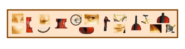
Bag-of-words model (BoW model) 最早出现在神经语言程序学(NLP)和信息检索（IR）领域. 该模型忽略掉文本的语法和语序, 用一组无序的单词(words)来表达一段文字或一个文档. 近年来, BoW模型被广泛应用于计算机视觉中. 与应用于文本的BoW类比, 图像的特征(feature)被当作单词(Word),把图像“文字化”之后，有助于大规模的图像检索.也有人把简写为Bag-of-Feature model(BOF model)或Bag-of-Visual-Word(BOVW model).
二、基本思想
1、提取特征：根据数据集选取特征，然后进行描述，形成特征数据，如检测图像中的sift keypoints,然后计算keypoints descriptors,生成128-D的特征向量；

2、学习词袋：利用处理好的特征数据全部合并，再用聚类的方法把特征词分为若干类，此若干类的数目由自己设定，每一个类相当于一个视觉词；

3、利用视觉词袋量化图像特征：每一张图像由很多视觉词汇组成，我们利用统计的词频直方图，可以表示图像属于哪一类。

三、关键步骤
1、特征描述（关键点提取）

在提取特征的时候，根据数据集选择特征，一般最流行的特征是sift、surf特征

SIFT特征
将一幅图像映射为一个局部特征向量集；特征向量具有平移、缩放、旋转不变性，同时对光照变化、仿射能让投影变换也有一定的不变性。

sift算法的特点：

1） SIFT特征是图像的局部特征，其对旋转、尺度缩放、亮度变化保持不变性，对视角变化、仿射变换、噪声也保持一定程度的稳定性；

2） 独特性（Distinctiveness）好，信息量丰富，适用于在海量特征数据库中进行快速、准确的匹配；

3） 多量性，即使少数的几个物体也可以产生大量的SIFT特征向量；

4） 高速性，经优化的SIFT匹配算法甚至可以达到实时的要求；

5） 可扩展性，可以很方便的与其他形式的特征向量进行联合。
2、聚类算法

K-means
1）计算每个聚类确定一个初始聚类中心，这样就可以有k个初始聚类中心

2）将样本集中的样本按照最小距离原则分配到最近邻聚类

3）使用每个聚类中的样本均值做为新的聚类中心直到聚类中心不再变化
四、相关代码及其实验结果
1、特征提取，生成词汇
import pickle
from PCV.imagesearch import vocabulary
from PCV.tools.imtools import get_imlist
from PCV.localdescriptors import sift

#获取图像列表
imlist = get_imlist(‘first1000/’)
nbr_images = len(imlist)
#获取特征列表
featlist = [imlist[i][:-3]+‘sift’ for i in range(nbr_images)]

#提取文件夹下图像的sift特征
for i in range(nbr_images):
sift.process_image(imlist[i], featlist[i])

#生成词汇
voc = vocabulary.Vocabulary(‘ukbenchtest’)
voc.train(featlist, 1000, 10)
#保存词汇

saving vocabulary

with open(‘first1000/vocabulary.pkl’, ‘wb’) as f:
pickle.dump(voc, f)
print (‘vocabulary is:’, voc.name, voc.nbr_words)

2、生成词汇字典

import pickle
from PCV.imagesearch import imagesearch
from PCV.localdescriptors import sift
from sqlite3 import dbapi2 as sqlite
from PCV.tools.imtools import get_imlist

#获取图像列表
imlist = get_imlist(‘first1000/’)
nbr_images = len(imlist)
#获取特征列表
featlist = [imlist[i][:-3]+‘sift’ for i in range(nbr_images)]

load vocabulary

#载入词汇
with open(‘first1000/vocabulary.pkl’, ‘rb’) as f:
voc = pickle.load(f)
#创建索引
indx = imagesearch.Indexer(‘testImaAdd.db’,voc)
indx.create_tables()

go through all images, project features on vocabulary and insert

#遍历所有的图像，并将它们的特征投影到词汇上
for i in range(nbr_images)[:1000]:
locs,descr = sift.read_features_from_file(featlist[i])
indx.add_to_index(imlist[i],descr)

commit to database

#提交到数据库
indx.db_commit()

con = sqlite.connect(‘testImaAdd.db’)
print (con.execute(‘select count (filename) from imlist’).fetchone())
print (con.execute(‘select * from imlist’).fetchone())

3、图片查询

-- coding: utf-8 --

import pickle
from PCV.localdescriptors import sift
from PCV.imagesearch import imagesearch
from PCV.geometry import homography
from PCV.tools.imtools import get_imlist

load image list and vocabulary

#载入图像列表
imlist = get_imlist(‘first1000/’)
nbr_images = len(imlist)
#载入特征列表
featlist = [imlist[i][:-3]+‘sift’ for i in range(nbr_images)]

#载入词汇
with open(‘first1000/vocabulary.pkl’, ‘rb’) as f:
voc = pickle.load(f)

src = imagesearch.Searcher(‘testImaAdd.db’,voc)

index of query image and number of results to return

#查询图像索引和查询返回的图像数
q_ind = 0
nbr_results = 20

regular query

常规查询(按欧式距离对结果排序)

res_reg = [w[1] for w in src.query(imlist[q_ind])[:nbr_results]]
print (‘top matches (regular):’, res_reg)

load image features for query image

#载入查询图像特征
q_locs,q_descr = sift.read_features_from_file(featlist[q_ind])
fp = homography.make_homog(q_locs[:,:2].T)

RANSAC model for homography fitting

#用单应性进行拟合建立RANSAC模型
model = homography.RansacModel()
rank = {}

load image features for result

#载入候选图像的特征
for ndx in res_reg[1:]:
locs,descr = sift.read_features_from_file(featlist[ndx]) # because ‘ndx’ is a rowid of the DB that starts at 1
# get matches
matches = sift.match(q_descr,descr)
ind = matches.nonzero()[0]
ind2 = matches[ind]
tp = homography.make_homog(locs[:,:2].T)
# compute homography, count inliers. if not enough matches return empty list
try:
H,inliers = homography.H_from_ransac(fp[:,ind],tp[:,ind2],model,match_theshold=4)
except:
inliers = []
# store inlier count
rank[ndx] = len(inliers)

sort dictionary to get the most inliers first

sorted_rank = sorted(rank.items(), key=lambda t: t[1], reverse=True)
res_geom = [res_reg[0]]+[s[0] for s in sorted_rank]
print (‘top matches (homography):’, res_geom)

显示查询结果

imagesearch.plot_results(src,res_reg[:8]) #常规查询
imagesearch.plot_results(src,res_geom[:8]) #重排后的结果
结果图：