5. 机器学习实战之逻辑回归处理UCI乳腺癌数据集
1. UCI Breast Cancer 数据集的下载途径
- Kaggle平台
https://www.kaggle.com/uciml/breast-cancer-wisconsin-data - UCI Machine Learning Repository
https://archive.ics.uci.edu/ml/datasets/Breast+Cancer+Wisconsin+%28Diagnostic%29 - Python Sklearn 的数据集
2. 数据探索
该数据集是从乳腺肿块的细针抽吸(FNA)的数字化图像计算特征。 它们描述了图像中存在的细胞核的特征。
属性信息:
1)身份证号码
2)诊断(M =恶性,B =良性)
3-32)
为每个细胞核计算十个实值特征:
a)半径(从中心到周长上的点的距离的平均值)
b)纹理(灰度值的标准偏差)
c)周长
d)面积
e)平滑度(半径长度的局部变化)
f)紧凑度(周长^ 2 /面积-1.0)
g)凹度(轮廓凹部的严重程度)
h)凹点(轮廓的凹入部分的数量)
i)对称
j)分形维数(“海岸线近似”-1)
from sklearn.datasets import load_breast_cancer
import pandas as pd
import matplotlib.pyplot as plt
import seaborn as sns
%matplotlib inline
data = load_breast_cancer()
data.keys()
dict_keys(['data', 'target', 'target_names', 'DESCR', 'feature_names', 'filename'])
train = pd.DataFrame(data.data, columns = data.feature_names)
train.head()
mean radius mean texture mean perimeter mean area mean smoothness mean compactness mean concavity mean concave points mean symmetry mean fractal dimension ... worst radius worst texture worst perimeter worst area worst smoothness worst compactness worst concavity worst concave points worst symmetry worst fractal dimension
0 17.99 10.38 122.80 1001.0 0.11840 0.27760 0.3001 0.14710 0.2419 0.07871 ... 25.38 17.33 184.60 2019.0 0.1622 0.6656 0.7119 0.2654 0.4601 0.11890
1 20.57 17.77 132.90 1326.0 0.08474 0.07864 0.0869 0.07017 0.1812 0.05667 ... 24.99 23.41 158.80 1956.0 0.1238 0.1866 0.2416 0.1860 0.2750 0.08902
2 19.69 21.25 130.00 1203.0 0.10960 0.15990 0.1974 0.12790 0.2069 0.05999 ... 23.57 25.53 152.50 1709.0 0.1444 0.4245 0.4504 0.2430 0.3613 0.08758
3 11.42 20.38 77.58 386.1 0.14250 0.28390 0.2414 0.10520 0.2597 0.09744 ... 14.91 26.50 98.87 567.7 0.2098 0.8663 0.6869 0.2575 0.6638 0.17300
4 20.29 14.34 135.10 1297.0 0.10030 0.13280 0.1980 0.10430 0.1809 0.05883 ... 22.54 16.67 152.20 1575.0 0.1374 0.2050 0.4000 0.1625 0.2364 0.07678
train.info()
<class 'pandas.core.frame.DataFrame'>
RangeIndex: 569 entries, 0 to 568
Data columns (total 30 columns):
mean radius 569 non-null float64
mean texture 569 non-null float64
mean perimeter 569 non-null float64
mean area 569 non-null float64
mean smoothness 569 non-null float64
mean compactness 569 non-null float64
mean concavity 569 non-null float64
mean concave points 569 non-null float64
mean symmetry 569 non-null float64
mean fractal dimension 569 non-null float64
radius error 569 non-null float64
texture error 569 non-null float64
perimeter error 569 non-null float64
area error 569 non-null float64
smoothness error 569 non-null float64
compactness error 569 non-null float64
concavity error 569 non-null float64
concave points error 569 non-null float64
symmetry error 569 non-null float64
fractal dimension error 569 non-null float64
worst radius 569 non-null float64
worst texture 569 non-null float64
worst perimeter 569 non-null float64
worst area 569 non-null float64
worst smoothness 569 non-null float64
worst compactness 569 non-null float64
worst concavity 569 non-null float64
worst concave points 569 non-null float64
worst symmetry 569 non-null float64
worst fractal dimension 569 non-null float64
dtypes: float64(30)
memory usage: 133.5 KB
train.describe()
mean radius mean texture mean perimeter mean area mean smoothness mean compactness mean concavity mean concave points mean symmetry mean fractal dimension ... worst radius worst texture worst perimeter worst area worst smoothness worst compactness worst concavity worst concave points worst symmetry worst fractal dimension
count 569.000000 569.000000 569.000000 569.000000 569.000000 569.000000 569.000000 569.000000 569.000000 569.000000 ... 569.000000 569.000000 569.000000 569.000000 569.000000 569.000000 569.000000 569.000000 569.000000 569.000000
mean 14.127292 19.289649 91.969033 654.889104 0.096360 0.104341 0.088799 0.048919 0.181162 0.062798 ... 16.269190 25.677223 107.261213 880.583128 0.132369 0.254265 0.272188 0.114606 0.290076 0.083946
std 3.524049 4.301036 24.298981 351.914129 0.014064 0.052813 0.079720 0.038803 0.027414 0.007060 ... 4.833242 6.146258 33.602542 569.356993 0.022832 0.157336 0.208624 0.065732 0.061867 0.018061
min 6.981000 9.710000 43.790000 143.500000 0.052630 0.019380 0.000000 0.000000 0.106000 0.049960 ... 7.930000 12.020000 50.410000 185.200000 0.071170 0.027290 0.000000 0.000000 0.156500 0.055040
25% 11.700000 16.170000 75.170000 420.300000 0.086370 0.064920 0.029560 0.020310 0.161900 0.057700 ... 13.010000 21.080000 84.110000 515.300000 0.116600 0.147200 0.114500 0.064930 0.250400 0.071460
50% 13.370000 18.840000 86.240000 551.100000 0.095870 0.092630 0.061540 0.033500 0.179200 0.061540 ... 14.970000 25.410000 97.660000 686.500000 0.131300 0.211900 0.226700 0.099930 0.282200 0.080040
75% 15.780000 21.800000 104.100000 782.700000 0.105300 0.130400 0.130700 0.074000 0.195700 0.066120 ... 18.790000 29.720000 125.400000 1084.000000 0.146000 0.339100 0.382900 0.161400 0.317900 0.092080
max 28.110000 39.280000 188.500000 2501.000000 0.163400 0.345400 0.426800 0.201200 0.304000 0.097440 ... 36.040000 49.540000 251.200000 4254.000000 0.222600 1.058000 1.252000 0.291000 0.663800 0.207500
8 rows × 30 columns
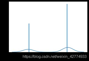
sns.distplot(train.target,bins =30)
plt.show()
逻辑回归
数据预处理
from sklearn.linear_model import LogisticRegression
from sklearn.model_selection import train_test_split
from sklearn.preprocessing import MinMaxScaler

#归一化预处理: 将有量纲变成无量纲,本案例用MinMaxScaler归一到0,1之间。从原理中我们注意到有一个axis=0,这表示MinMaxScaler方法默认是对每一列做这样的归一化操作,这也比较符合实际应用。(MaxAbsScaler:归一到 [ -1,1 ] )
#StandardScaler是标准化,去均值和方差归一化。针对每一个特征维度(列)来做的,而不是针对样本
#Normalize/Normalizer 正则化 针对每一个样本来做, 有L1, L2 范数。正则化的过程是将每个样本缩放到单位范数(每个样本的范数为1),如果后面要使用如二次型(点积)或者其它核方法计算两个样本之间的相似性这个方法会很有用。该方法主要应用于文本分类和聚类中;

data_X = train.drop(columns ='target')
data_y = train.target
scaler = MinMaxScaler()
scaler.fit(data_X)
print(scaler.data_max_)
scaler.transform(data_X)

train_X, test_X, train_y, test_y = train_test_split(data_X, data_y, test_size = 0.25, random_state = 666)
训练
逻辑回归的参数
#LogisticRegression(
#     penalty='l2',
#     dual=False,
#     tol=0.0001,
#     C=1.0,
#     fit_intercept=True,
#     intercept_scaling=1,
#     class_weight=None,
#     random_state=None,
#     solver='lbfgs',
#     max_iter=100,
#     multi_class='auto',
#     verbose=0,
#     warm_start=False,
#     n_jobs=None,
#     l1_ratio=None,
# )

# penalty: penalty参数可选择的值为”l1”和”l2”.分别对应L1的正则化和L2的正则化,默认是L2的正则化。调参时如果我们主要的目的只是为了解决过拟合,一般penalty选择L2正则化就够了。但是如果选择L2正则化发现还是过拟合,即预测效果差的时候,就可以考虑L1正则化。另外,如果模型的特征非常多,我们希望一些不重要的特征系数归零,从而让模型系数稀疏化的话,也可以使用L1正则化。
# solver : 损失函数优化算法。 penalty参数的选择会影响我们损失函数优化算法的选择。即参数solver的选择,如果是L2正则化,那么4种可选的算法{‘newton-cg’, ‘lbfgs’, ‘liblinear’, ‘sag’}都可以选择。但是如果penalty是L1正则化的话,就只能选择‘liblinear’了。这是因为L1正则化的损失函数不是连续可导的,而{‘newton-cg’, ‘lbfgs’,‘sag’}这三种优化算法时都需要损失函数的一阶或者二阶连续导数。而‘liblinear’并没有这个依赖。

# C: C为正则化系数λ的倒数,通常默认为1
#fit_intercept : 是否存在截距,默认存在
具体参考
http://scikit-learn.org/stable/modules/generated/sklearn.linear_model.LogisticRegression.html
LR = LogisticRegression(verbose = 0,random_state = 666)
LR.fit(train_X, train_y)

LogisticRegression(C=1.0, class_weight=None, dual=False, fit_intercept=True,
                   intercept_scaling=1, l1_ratio=None, max_iter=100,
                   multi_class='auto', n_jobs=None, penalty='l2',
                   random_state=666, solver='lbfgs', tol=0.0001, verbose=0,
                   warm_start=False)

print(LR.coef_ , LR.intercept_ , LR.n_iter_)
[[ 0.68347194  0.44483351  0.44744758 -0.02074153 -0.02036978 -0.11193005
  -0.15194855 -0.06504914 -0.0253229  -0.00643472  0.03397449  0.305727
   0.11109548 -0.11448631 -0.00250216 -0.02674393 -0.03244407 -0.00857176
  -0.00824784 -0.00244437  0.70605004 -0.48033477 -0.31624411 -0.010282
  -0.03918421 -0.34941889 -0.41463748 -0.12604286 -0.10172979 -0.03386901]] [0.12201617] [100]

LR.predict(test_X)
array([0, 1, 1, 1, 0, 0, 0, 1, 0, 1, 1, 1, 1, 1, 1, 1, 1, 1, 1, 1, 0, 1,
       1, 1, 1, 1, 1, 0, 1, 0, 0, 1, 1, 0, 0, 1, 1, 0, 0, 1, 0, 1, 0, 1,
       1, 0, 1, 1, 0, 1, 1, 0, 0, 1, 1, 0, 0, 1, 1, 0, 1, 1, 1, 0, 1, 1,
       1, 0, 0, 0, 1, 1, 0, 1, 1, 1, 1, 1, 0, 0, 0, 0, 0, 1, 0, 0, 1, 0,
       1, 1, 1, 1, 1, 0, 1, 1, 0, 1, 0, 1, 1, 0, 0, 1, 0, 1, 0, 0, 1, 1,
       0, 1, 1, 0, 1, 1, 0, 1, 0, 1, 1, 1, 1, 1, 0, 1, 1, 1, 1, 1, 1, 0,
       0, 1, 1, 1, 1, 0, 0, 1, 0, 0, 0])
LR.predict_proba(test_X)
array([[9.99999777e-01, 2.22669515e-07],
       [1.65868346e-02, 9.83413165e-01],
       [3.73219760e-03, 9.96267802e-01],
       [1.67199408e-01, 8.32800592e-01],
       [9.99891516e-01, 1.08484106e-04],
       [9.91925024e-01, 8.07497597e-03],
       [9.98260573e-01, 1.73942655e-03],
       [4.18072481e-02, 9.58192752e-01],
       [9.99325497e-01, 6.74502859e-04],
       [1.53350004e-02, 9.84665000e-01],
       [8.96783706e-04, 9.99103216e-01],
       [7.35966445e-02, 9.26403355e-01],
       [4.02066133e-03, 9.95979339e-01],
       [3.50849048e-01, 6.49150952e-01],
       [4.40960629e-02, 9.55903937e-01],
       [7.45785996e-04, 9.99254214e-01],
       [1.16424472e-03, 9.98835755e-01],
       [5.97028048e-03, 9.94029720e-01],
       [5.27591728e-03, 9.94724083e-01],
       [3.45588825e-02, 9.65441117e-01],
       [9.78445197e-01, 2.15548029e-02],
       [2.91764970e-01, 7.08235030e-01],
       [3.45838547e-04, 9.99654161e-01],
       [1.14226423e-01, 8.85773577e-01],
       [9.45367169e-03, 9.90546328e-01],
       [2.49975998e-02, 9.75002400e-01],
       [1.07317628e-03, 9.98926824e-01],
       [1.00000000e+00, 2.36930376e-16],
       [4.23124322e-03, 9.95768757e-01],
       [1.00000000e+00, 8.45641190e-17],
       [9.98263097e-01, 1.73690281e-03],
       [5.49792340e-03, 9.94502077e-01],
       [3.49642972e-03, 9.96503570e-01],
       [1.00000000e+00, 4.51253397e-16],
       [9.99999996e-01, 3.84375926e-09],
       [2.85705764e-02, 9.71429424e-01],
       [5.12061111e-03, 9.94879389e-01],
       [9.99999997e-01, 2.85647392e-09],
       [9.99999601e-01, 3.98641153e-07],
       [7.41913052e-03, 9.92580869e-01],
       [9.62334921e-01, 3.76650788e-02],
       [4.24620296e-02, 9.57537970e-01],
       [1.00000000e+00, 7.06045821e-13],
       [3.89620167e-03, 9.96103798e-01],
       [4.76647919e-03, 9.95233521e-01],
       [9.99999999e-01, 8.96392848e-10],
       [7.05135419e-03, 9.92948646e-01],
       [1.22553741e-02, 9.87744626e-01],
       [9.99999979e-01, 2.11395049e-08],
       [6.33223741e-04, 9.99366776e-01],
       [1.37972662e-01, 8.62027338e-01],
       [9.99999980e-01, 2.03490893e-08],
       [1.00000000e+00, 2.48435212e-11],
       [2.82499431e-03, 9.97175006e-01],
       [5.70907727e-03, 9.94290923e-01],
       [9.99999684e-01, 3.15930037e-07],
       [9.79432533e-01, 2.05674668e-02],
       [1.83545873e-01, 8.16454127e-01],
       [6.68440757e-03, 9.93315592e-01],
       [9.82751351e-01, 1.72486487e-02],
       [5.54118416e-04, 9.99445882e-01],
       [2.02672896e-01, 7.97327104e-01],
       [2.09124523e-01, 7.90875477e-01],
       [9.99998174e-01, 1.82627830e-06],
       [4.76326253e-04, 9.99523674e-01],
       [8.46701224e-04, 9.99153299e-01],
       [3.84709365e-03, 9.96152906e-01],
       [5.47272438e-01, 4.52727562e-01],
       [1.00000000e+00, 4.88010481e-13],
       [9.99999631e-01, 3.69389221e-07],
       [5.05386347e-04, 9.99494614e-01],
       [5.12991025e-03, 9.94870090e-01],
       [9.99801111e-01, 1.98889168e-04],
       [5.51494923e-02, 9.44850508e-01],
       [4.46014260e-01, 5.53985740e-01],
       [2.07037506e-04, 9.99792962e-01],
       [2.31530770e-02, 9.76846923e-01],
       [4.72099180e-01, 5.27900820e-01],
       [6.86974372e-01, 3.13025628e-01],
       [9.99999972e-01, 2.79227956e-08],
       [1.00000000e+00, 5.86761671e-11],
       [9.99999981e-01, 1.94357371e-08],
       [9.99999538e-01, 4.62442532e-07],
       [3.46153087e-03, 9.96538469e-01],
       [1.00000000e+00, 1.07682200e-25],
       [8.99668025e-01, 1.00331975e-01],
       [1.87049526e-03, 9.98129505e-01],
       [9.99441195e-01, 5.58804721e-04],
       [2.28397639e-04, 9.99771602e-01],
       [2.44360002e-04, 9.99755640e-01],
       [4.27812775e-03, 9.95721872e-01],
       [5.18389948e-03, 9.94816101e-01],
       [1.10794137e-02, 9.88920586e-01],
       [1.00000000e+00, 8.13924218e-13],
       [3.44982827e-03, 9.96550172e-01],
       [6.54051148e-02, 9.34594885e-01],
       [9.99603964e-01, 3.96036481e-04],
       [9.26396881e-04, 9.99073603e-01],
       [6.43266635e-01, 3.56733365e-01],
       [2.59017709e-01, 7.40982291e-01],
       [1.99461805e-02, 9.80053819e-01],
       [1.00000000e+00, 4.75819615e-11],
       [9.99998814e-01, 1.18585849e-06],
       [1.36730728e-03, 9.98632693e-01],
       [9.99975923e-01, 2.40765881e-05],
       [4.06354422e-02, 9.59364558e-01],
       [9.99998050e-01, 1.95018517e-06],
       [1.00000000e+00, 3.17309299e-12],
       [5.29263458e-04, 9.99470737e-01],
       [2.07489011e-02, 9.79251099e-01],
       [9.86669602e-01, 1.33303979e-02],
       [4.24123363e-01, 5.75876637e-01],
       [2.26957551e-03, 9.97730424e-01],
       [9.99509316e-01, 4.90683993e-04],
       [1.49858020e-02, 9.85014198e-01],
       [1.82176647e-01, 8.17823353e-01],
       [9.99975521e-01, 2.44791952e-05],
       [6.31817306e-03, 9.93681827e-01],
       [7.70108042e-01, 2.29891958e-01],
       [1.34450222e-01, 8.65549778e-01],
       [2.18146065e-03, 9.97818539e-01],
       [8.17373367e-03, 9.91826266e-01],
       [5.40648477e-02, 9.45935152e-01],
       [2.78893419e-01, 7.21106581e-01],
       [9.99999995e-01, 5.37606891e-09],
       [8.85888230e-04, 9.99114112e-01],
       [9.49758147e-03, 9.90502419e-01],
       [6.23472937e-04, 9.99376527e-01],
       [4.29447729e-03, 9.95705523e-01],
       [7.61696199e-04, 9.99238304e-01],
       [4.75535700e-04, 9.99524464e-01],
       [9.99875475e-01, 1.24525042e-04],
       [9.95612659e-01, 4.38734098e-03],
       [7.41547622e-03, 9.92584524e-01],
       [5.17181654e-02, 9.48281835e-01],
       [2.35783150e-03, 9.97642168e-01],
       [1.01172987e-02, 9.89882701e-01],
       [1.00000000e+00, 9.65916831e-13],
       [9.99996236e-01, 3.76386483e-06],
       [1.13847391e-02, 9.88615261e-01],
       [1.00000000e+00, 3.65023905e-13],
       [8.55769403e-01, 1.44230597e-01],
       [8.66364202e-01, 1.33635798e-01]])

LR.score(train_X,train_y)
0.9530516431924881
LR.score(test_X,test_y)
0.9370629370629371
混淆矩阵
from sklearn.metrics import confusion_matrix, f1_score

print(confusion_matrix(test_y, pred_y))
print(f1_score(test_y,pred_y))
[[51  5]
 [ 4 83]]
0.9485714285714286
交叉验证 可以在数据量很少的情况下 提高训练效率
from sklearn.model_selection import cross_val_score,cross_val_predict, KFold

LR = LogisticRegression(verbose = 0,random_state = 666)
scores =cross_val_score(LR, train_X, train_y, cv=3)

print(scores.mean())
print(scores)
0.9530516431924881
array([0.94366197, 0.96478873, 0.95070423])
cross_val_score: 对数据集进行指定次数的交叉验证并为每次验证效果评测. 其中,score 默认是以 scoring='f1_macro’进行评测
cross_val_predict: 与cross_val_score 很相像,不过不同于返回的是评测效果,cross_val_predict 返回的是estimator 的分类结果(或回归值)
KFold : K折交叉验证,这是将数据集分成K份的官方给定方案,所谓K折就是将数据集通过K次分割,使得所有数据既在训练集出现过,又在测试集出现过,当然,每次分割中不会有重叠。相当于无放回抽样。
更多模型评估可以参考
https://scikit-learn.org/stable/modules/model_evaluation.html
http://scikit-learn.org/stable/modules/cross_validation.html