faster-rcnn算法总结

代码git地址：https://github.com/endernewton/tf-faster-rcnn

原理解读

​ R-CNN --> FAST-RCNN --> FASTER-RCNN

R-CNN:

(1)输入测试图像；

(2)利用selective search 算法在图像中从上到下提取2000个左右的Region Proposal；

(3)将每个Region Proposal缩放(warp)成227*227的大小并输入到CNN，将CNN的fc7层的输出作为特征；

(4)将每个Region Proposal提取的CNN特征输入到SVM进行分类；

(5)对于SVM分好类的Region Proposal做边框回归，用Bounding box回归值校正原来的建议窗口，生成预测窗口坐标.

缺陷:

(1) 训练分为多个阶段，步骤繁琐：微调网络+训练SVM+训练边框回归器；

(2) 训练耗时，占用磁盘空间大；5000张图像产生几百G的特征文件；

(3) 速度慢：使用GPU，VGG16模型处理一张图像需要47s；

(4) 测试速度慢：每个候选区域需要运行整个前向CNN计算；

(5) SVM和回归是事后操作，在SVM和回归过程中CNN特征没有被学习更新.

FAST-RCNN:

(1)输入测试图像；

(2)利用selective search 算法在图像中从上到下提取2000个左右的建议窗口(Region Proposal)；

(3)将整张图片输入CNN，进行特征提取；

(4)把建议窗口映射到CNN的最后一层卷积feature map上；

(5)通过RoI pooling层使每个建议窗口生成固定尺寸的feature map；

(6)利用Softmax Loss(探测分类概率) 和Smooth L1 Loss(探测边框回归)对分类概率和边框回归(Bounding box regression)联合训练.

相比R-CNN，主要两处不同:

(1)最后一层卷积层后加了一个ROI pooling layer；

(2)损失函数使用了多任务损失函数(multi-task loss)，将边框回归直接加入到CNN网络中训练

改进:

(1) 测试时速度慢：R-CNN把一张图像分解成大量的建议框，每个建议框拉伸形成的图像都会单独通过CNN提取特征.实际上这些建议框之间大量重叠，特征值之间完全可以共享，造成了运算能力的浪费.

FAST-RCNN将整张图像归一化后直接送入CNN，在最后的卷积层输出的feature map上，加入建议框信息，使得在此之前的CNN运算得以共享.

(2) 训练时速度慢：R-CNN在训练时，是在采用SVM分类之前，把通过CNN提取的特征存储在硬盘上.这种方法造成了训练性能低下，因为在硬盘上大量的读写数据会造成训练速度缓慢.

FAST-RCNN在训练时，只需要将一张图像送入网络，每张图像一次性地提取CNN特征和建议区域，训练数据在GPU内存里直接进Loss层，这样候选区域的前几层特征不需要再重复计算且不再需要把大量数据存储在硬盘上.

(3) 训练所需空间大：R-CNN中独立的SVM分类器和回归器需要大量特征作为训练样本，需要大量的硬盘空间.FAST-RCNN把类别判断和位置回归统一用深度网络实现，不再需要额外存储.

FASTER -RCNN:

整体架构：

(1)输入测试图像；

(2)将整张图片输入CNN，进行特征提取；

(3)用RPN生成建议窗口(proposals)，每张图片生成300个建议窗口；

(4)把建议窗口映射到CNN的最后一层卷积feature map上；

(5)通过RoI pooling层使每个RoI生成固定尺寸的feature map；

(6)利用Softmax Loss(探测分类概率) 和Smooth L1 Loss(探测边框回归)对分类概率和边框回归(Bounding box regression)联合训练.

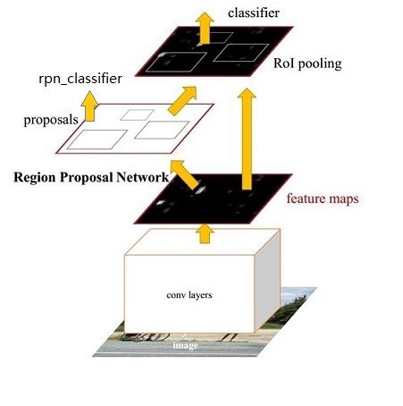
我们先整体的介绍下上图中各层主要的功能

1)、Conv layers提取特征图：

作为一种CNN网络目标检测方法，Faster RCNN首先使用一组基础的conv+relu+pooling层提取input image的feature maps,该feature maps会用于后续的RPN层和全连接层

2)、RPN(Region Proposal Networks):

​ RPN网络主要用于生成region proposals，首先生成一堆Anchor box，对其进行裁剪过滤后通过softmax判断anchors属于前景(foreground)或者后景(background)，即是物体or不是物体，所以这是一个二分类；同时，另一分支bounding box regression修正anchor box，形成较精确的proposal（注：这里的较精确是相对于后面全连接层的再一次box regression而言）

3)、Roi Pooling：

该层利用RPN生成的proposals和VGG16最后一层得到的feature map，得到固定大小的proposal feature map,进入到后面可利用全连接操作来进行目标识别和定位

4)、Classifier：

​ 会将Roi Pooling层形成固定大小的feature map进行全连接操作，利用Softmax进行具体类别的分类，同时，利用L1 Loss完成bounding box regression回归操作获得物体的精确位置.

相比FASTER-RCNN，主要两处不同:

(1)使用RPN(Region Proposal Network)代替原来的Selective Search方法产生建议窗口；

(2)产生建议窗口的CNN和目标检测的CNN共享

改进:

(1) 如何高效快速产生建议框？

FASTER-RCNN创造性地采用卷积网络自行产生建议框，并且和目标检测网络共享卷积网络，使得建议框数目从原有的约2000个减少为300个，且建议框的质量也有本质的提高.

网络结构

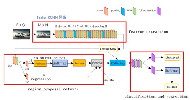
现在，通过上图开始逐层分析

Conv layers

Faster RCNN首先是支持输入任意大小的图片的，比如上图中输入的P*Q，进入网络之前对图片进行了规整化尺度的设定，如可设定图像短边不超过600，图像长边不超过1000，我们可以假定M*N=1000*600（如果图片少于该尺寸，可以边缘补0，即图像会有黑色边缘）

① 13个conv层：kernel_size=3,pad=1,stride=1;

卷积公式：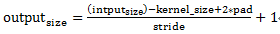

​ 所以，conv层不会改变图片大小（即：输入的图片大小=输出的图片大小）

② 13个relu层：激活函数，不改变图片大小

③ 4个pooling层：kernel_size=2,stride=2;pooling层会让输出图片是输入图片的1/2

​ 经过Conv layers，图片大小变成(M/16)*(N/16)，即：60*40(1000/16≈60,600/16≈40)；则，Feature Map就是60*40*512-d(注：VGG16是512-d,ZF是256-d)，表示特征图的大小为60*40，数量为512

RPN(Region Proposal Networks):

Feature Map进入RPN后，先经过一次3*3的卷积，同样，特征图大小依然是60*40,数量512，这样做的目的应该是进一步集中特征信息，接着看到两个全卷积,即kernel_size=1*1,p=0,stride=1;

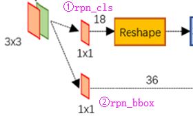
如上图中标识：

① rpn_cls：60*40*512-d ⊕ 1*1*512*18 ==> 60*40*9*2

​ 逐像素对其9个Anchor box进行二分类

② rpn_bbox：60*40*512-d ⊕ 1*1*512*36==>60*40*9*4

​ 逐像素得到其9个Anchor box四个坐标信息（其实是偏移量，后面介绍）

如下图所示：

(2.1)、Anchors的生成规则

​ 前面提到经过Conv layers后，图片大小变成了原来的1/16，令_feat_stride=16，在生成Anchors时，我们先定义一个base_anchor，大小为16*16的box(因为特征图(60*40)上的一个点，可以对应到原图（1000*600）上一个16*16大小的区域)，源码中转化为[0,0,15,15]的数组，参数ratios=[0.5, 1, 2],scales=[8, 16, 32]

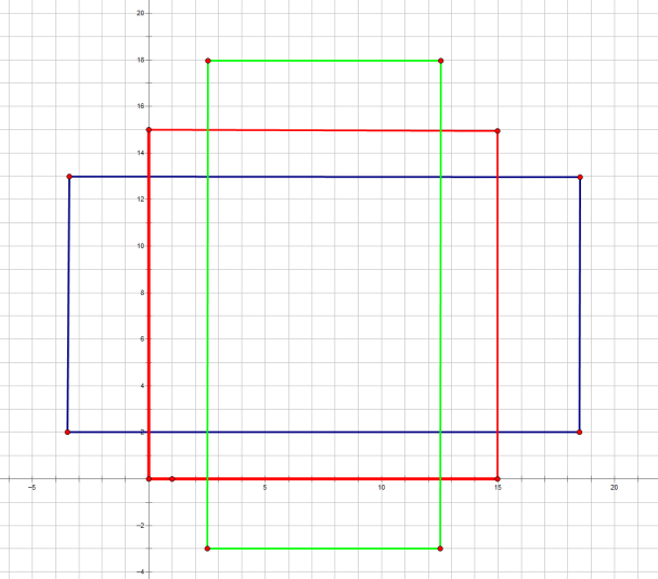
先看[0,0,15,15],面积保持不变，长、宽比分别为[0.5, 1, 2]是产生的Anchors box

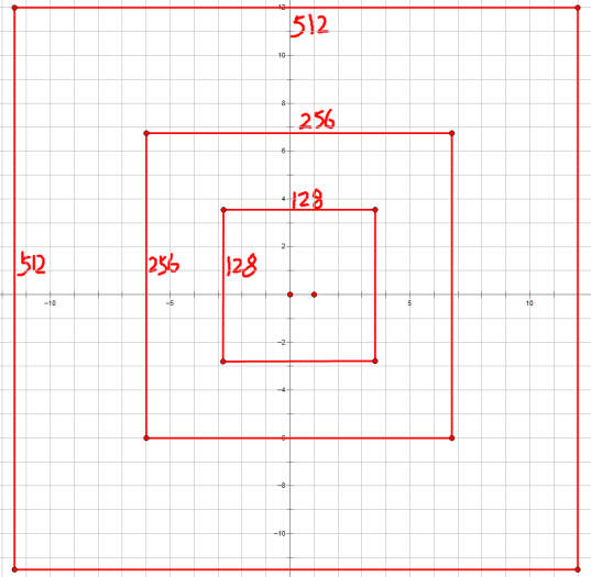
如果经过scales变化，即长、宽分别均为 (16*8=128)、(16*16=256)、(16*32=512)，对应anchor box如图

综合以上两种变换，最后生成9个Anchor box

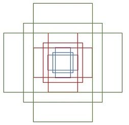
所以，最终base_anchor=[0,0,15,15]生成的9个Anchor box坐标如下：

[](javascript:void(0)?

1 [[ -84.  -40.   99.   55.]  
2 [-176.  -88.  191.  103.]  
3 [-360. -184.  375.  199.]  
4 [ -56.  -56.   71.   71.]  
5 [-120. -120.  135.  135.]  
6 [-248. -248.  263.  263.]  
7 [ -36.  -80.   51.   95.]  
8 [ -80. -168.   95.  183.]  
9 [-168. -344.  183.  359.]] 

[](javascript:void(0)?

​ 特征图大小为60*40，所以会一共生成60*40*9=21600个Anchor box

源码中，通过width:(0-60)*16,height(0-40)*16建立shift偏移量数组，再和base_anchor基准坐标数组累加，得到特征图上所有像素对应的Anchors的坐标值，是一个[216000,4]的数组

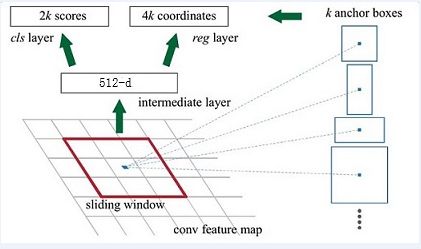
RPN的实现方式：在conv5-3的卷积feature map上用一个n*n的滑窗（论文中作者选用了n=3，即3*3的滑窗）生成一个长度为256（对应于ZF网络）或512（对应于VGG网络）维长度的全连接特征.然后在这个256维或512维的特征后产生两个分支的全连接层：

(1)reg-layer,用于预测proposal的中心锚点对应的proposal的坐标x，y和宽高w，h；

(2)cls-layer，用于判定该proposal是前景还是背景.sliding window的处理方式保证reg-layer和cls-layer关联了conv5-3的全部特征空间.事实上，作者用全连接层实现方式介绍RPN层实现容易帮助我们理解这一过程，但在实现时作者选用了卷积层实现全连接层的功能.

(3)个人理解：全连接层本来就是特殊的卷积层，如果产生256或512维的fc特征，事实上可以用Num_out=256或512, kernel_size=3*3, stride=1的卷积层实现conv5-3到第一个全连接特征的映射.然后再用两个Num_out分别为2*9=18和4*9=36，kernel_size=1*1，stride=1的卷积层实现上一层特征到两个分支cls层和reg层的特征映射.

(4)注意：这里2*9中的2指cls层的分类结果包括前后背景两类，4*9的4表示一个Proposal的中心点坐标x，y和宽高w，h四个参数.采用卷积的方式实现全连接处理并不会减少参数的数量，但是使得输入图像的尺寸可以更加灵活.在RPN网络中，我们需要重点理解其中的anchors概念，Loss fucntions计算方式和RPN层训练数据生成的具体细节.

Anchors:字面上可以理解为锚点，位于之前提到的n*n的sliding window的中心处.对于一个sliding window,我们可以同时预测多个proposal，假定有k个proposal即k个reference boxes，每一个reference box又可以用一个scale，一个aspect_ratio和sliding window中的锚点唯一确定.所以，我们在后面说一个anchor,你就理解成一个anchor box 或一个reference box.作者在论文中定义k=9，即3种scales和3种aspect_ratio确定出当前sliding window位置处对应的9个reference boxes， 4*k个reg-layer的输出和2*k个cls-layer的score输出.对于一幅W*H的feature map,对应W*H*k个锚点.所有的锚点都具有尺度不变性.

Loss functions:

在计算Loss值之前，作者设置了anchors的标定方法.正样本标定规则：

1. 如果Anchor对应的reference box与ground truth的IoU值最大，标记为正样本；

2. 如果Anchor对应的reference box与ground truth的IoU>0.7，标记为正样本.事实上，采用第2个规则基本上可以找到足够的正样本，但是对于一些极端情况，例如所有的Anchor对应的reference box与groud truth的IoU不大于0.7,可以采用第一种规则生成.

3. 负样本标定规则：如果Anchor对应的reference box与ground truth的IoU<0.3，标记为负样本.

4. 剩下的既不是正样本也不是负样本，不用于最终训练.

5. 训练RPN的Loss是有classification loss （即softmax loss）和regression loss （即L1 loss）按一定比重组成的.

计算softmax loss需要的是anchors对应的groundtruth标定结果和预测结果，计算regression loss需要三组信息：

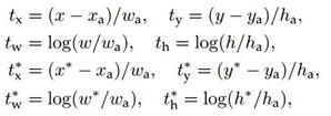
i. 预测框，即RPN网络预测出的proposal的中心位置坐标x,y和宽高w,h；

ii. 锚点reference box:

​ 之前的9个锚点对应9个不同scale和aspect_ratio的reference boxes，每一个reference boxes都有一个中心点位置坐标x_a,y_a和宽高w_a,h_a；

iii. ground truth:标定的框也对应一个中心点位置坐标x*,y和宽高w,h*.因此计算regression loss和总Loss方式如下：

RPN训练设置：

(1)在训练RPN时，一个Mini-batch是由一幅图像中任意选取的256个proposal组成的，其中正负样本的比例为1：1.

(2)如果正样本不足128，则多用一些负样本以满足有256个Proposal可以用于训练，反之亦然.

(3)训练RPN时，与VGG共有的层参数可以直接拷贝经ImageNet训练得到的模型中的参数；剩下没有的层参数用标准差=0.01的高斯分布初始化.

• RPN工作原理解析

为了进一步更清楚的看懂RPN的工作原理，将Caffe版本下的网络图贴出来，对照网络图进行讲解会更清楚

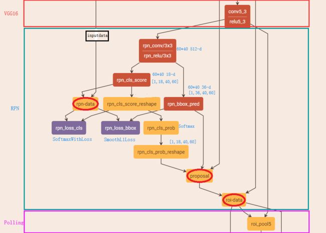
主要看上图中框住的‘RPN’部分的网络图，其中‘rpn_conv/3*3’是3*3的卷积，上面有提到过，接着是两个1*1的全卷积，分别是图中的‘rpn_cls_score’和‘rpn_bbox_pred’，在上面同样有提到过。接下来，分析网络图中其他各部分的含义

rpn-data:

为特征图60*40上的每个像素生成9个Anchor box，并且对生成的Anchor box进行过滤和标记，参照源码，过滤和标记规则如下：

① 去除掉超过1000*600这原图的边界的anchor box

② 如果anchor box与ground truth的IoU值最大，标记为正样本，label=1

③ 如果anchor box与ground truth的IoU>0.7，标记为正样本，label=1

④ 如果anchor box与ground truth的IoU<0.3，标记为负样本，label=0

​ 剩下的既不是正样本也不是负样本，不用于最终训练，label=-1

​ 除了对anchor box进行标记外，另一件事情就是计算anchor box与ground truth之间的偏移量

令：ground truth:标定的框也对应一个中心点位置坐标x*,y和宽高w,h*

​ anchor box: 中心点位置坐标x_a,y_a和宽高w_a,h_a

​ 所以，偏移量：

​ △x=(x-x_a)/w_a △y=(y-y_a)/h_a

△w=log(w/w_a) △h=log(h*/h_a)

​ 通过ground truth box与预测的anchor box之间的差异来进行学习，从而是RPN网络中的权重能够学习到预测box的能力

rpn_loss_cls、rpn_loss_bbox、rpn_cls_prob:

下面集体看下这三个，其中‘rpn_loss_cls’、‘rpn_loss_bbox’是分别对应softmax，smooth L1计算损失函数，‘rpn_cls_prob’计算概率值(可用于下一层的nms非最大值抑制操作)

补充：

​ ① Softmax公式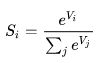，计算各分类的概率值

​ ② Softmax Loss公式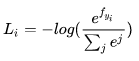，RPN进行分类时，即寻找最小Loss值

在’rpn-data’中已经为预测框anchor box进行了标记，并且计算出与gt_boxes之间的偏移量,利用RPN网络进行训练。

RPN训练设置：在训练RPN时，一个Mini-batch是由一幅图像中任意选取的256个proposal组成的，其中正负样本的比例为1：1。如果正样本不足128，则多用一些负样本以满足有256个Proposal可以用于训练，反之亦然

proposal：

’rpn_bbox_pred’，记录着训练好的四个回归值△x, △y, △w, △h。

源码中，会重新生成60*40*9个anchor box，然后累加上训练好的△x, △y, △w, △h,从而得到了相较于之前更加准确的预测框region proposal，进一步对预测框进行越界剔除和使用nms非最大值抑制，剔除掉重叠的框；比如，设定IoU为0.7的阈值，即仅保留覆盖率不超过0.7的局部最大分数的box（粗筛）。最后留下大约2000个anchor，然后再取前N个box（比如300个）；这样，进入到下一层ROI Pooling时region proposal大约只有300个

roi_data：

为了避免定义上的误解，我们将经过‘proposal’后的预测框称为region proposal（其实，RPN层的任务其实已经完成，roi_data属于为下一层准备数据）

主要作用：

① RPN层只是来确定region proposal是否是物体(是/否),这里根据region proposal和ground truth box的最大重叠指定具体的标签(就不再是二分类问题了，参数中指定的是81类)

② 计算region proposal与ground truth boxes的偏移量，计算方法和之前的偏移量计算公式相同

经过这一步后的数据输入到ROI Pooling层进行进一步的分类和定位.

ROI Pooling

这层输入的是RPN层产生的region proposal(假定有300个region proposal box)和VGG16最后一层产生的特征图(60*40* 512-d)，遍历每个region proposal，将其坐标值缩小16倍，这样就可以将在原图(1000*600)基础上产生的region proposal映射到60*40的特征图上，从而将在feature map上确定一个区域(定义为RB)。

在feature map上确定的区域RB，根据参数pooled_w:7,pooled_h:7,将这个RB区域划分为7*7，即49个相同大小的小区域，对于每个小区域，使用max pooling方式从中选取最大的像素点作为输出，这样，就形成了一个7*7的feature map

以此，参照上述方法，300个region proposal遍历完后，会产生很多个7*7大小的feature map，故而输出的数组是：[300,512,7,7],作为下一层的全连接的输入

ROI pooling layer实际上是SPP-NET的一个精简版，SPP-NET对每个proposal使用了不同大小的金字塔映射，而ROI pooling layer只需要下采样到一个7x7的特征图.对于VGG16网络conv5_3有512个特征图，这样所有region proposal对应了一个7*7*512维度的特征向量作为全连接层的输入.

RoI Pooling就是实现从原图区域映射到conv5区域最后pooling到固定大小的功能.

全连接层

经过roi pooling层之后，batch_size=300, proposal feature map的大小是7*7,512-d,对特征图进行全连接，参照下图，最后同样利用Softmax Loss和L1 Loss完成分类和定位

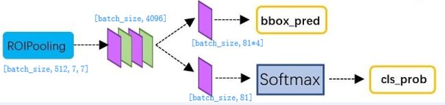
通过full connect层与softmax计算每个region proposal具体属于哪个类别（如人，马，车等），输出cls_prob概率向量；同时再次利用bounding box regression获得每个region proposal的位置偏移量bbox_pred，用于回归获得更加精确的目标检测框

即从PoI Pooling获取到7x7大小的proposal feature maps后，通过全连接主要做了：

4.1)通过全连接和softmax对region proposals进行具体类别的分类

4.2)再次对region proposals进行bounding box regression，获取更高精度的rectangle box

概念解释：

SPP-NET

SSP-Net：Spatial Pyramid Pooling in Deep Convolutional Networks for Visual Recognition

先看一下R-CNN为什么检测速度这么慢，一张图都需要47s！仔细看下R-CNN框架发现，对图像提完Region Proposal（2000个左右）之后将每个Proposal当成一张图像进行后续处理(CNN提特征+SVM分类)，实际上对一张图像进行了2000次提特征和分类的过程！这2000个Region Proposal不都是图像的一部分吗，那么我们完全可以对图像提一次卷积层特征，然后只需要将Region Proposal在原图的位置映射到卷积层特征图上，这样对于一张图像我们只需要提一次卷积层特征，然后将每个Region Proposal的卷积层特征输入到全连接层做后续操作.（对于CNN来说，大部分运算都耗在卷积操作上，这样做可以节省大量时间）.

现在的问题是每个Region Proposal的尺度不一样，直接这样输入全连接层肯定是不行的，因为全连接层输入必须是固定的长度.SPP-NET恰好可以解决这个问题.

​

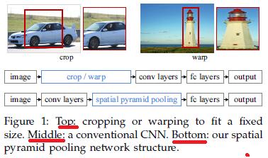
由于传统的CNN限制了输入必须固定大小（比如AlexNet是224x224），所以在实际使用中往往需要对原图片进行crop或者warp的操作：

• crop：截取原图片的一个固定大小的patch(物体可能会产生截断，尤其是长宽比大的图片)

• warp：将原图片的ROI缩放到一个固定大小的patch(物体被拉伸，失去“原形”，尤其是长宽比大的图片)

  SPP为的就是解决上述的问题，做到的效果为：不管输入的图片是什么尺度，都能够正确的传入网络.
  具体思路为：CNN的卷积层是可以处理任意尺度的输入的，只是在全连接层处有限制尺度——换句话说，如果找到一个方法，在全连接层之前将其输入限制到等长，那么就解决了这个问题.

  具体方案如下图所示：

  

如果原图输入是224x224，对于conv5出来后的输出，是13x13x256的，可以理解成有256个这样的filter，每个filter对应一张13x13的activation map.如果像上图那样将activation map pooling成4x4、2x2、1x1三张子图，做max pooling后，出来的特征就是固定长度的(16+4+1)x256那么多的维度了.如果原图的输入不是224x224，出来的特征依然是(16+4+1)x256；直觉地说，可以理解成将原来固定大小为(3x3)窗口的pool5改成了自适应窗口大小，窗口的大小和activation map成比例，保证了经过pooling后出来的feature的长度是一致的.

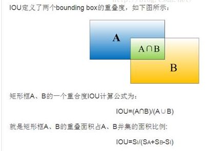
IOU

​

​ 除了对anchor box进行标记外，另一件事情就是计算anchor box与ground truth之间的偏移量

令：ground truth:标定的框也对应一个中心点位置坐标x*,y和宽高w,h*

​ anchor box: 中心点位置坐标x_a,y_a和宽高w_a,h_a

​ 所以，偏移量：

​ △x=(x-x_a)/w_a △y=(y*-y_a)/h_a

△w=log(w/w_a) △h=log(h*/h_a)

​ 通过ground truth box与预测的anchor box之间的差异来进行学习，从而是RPN网络中的权重能够学习到预测box的能力

NMS

用下图一个案例来对NMS算法进行简单介绍

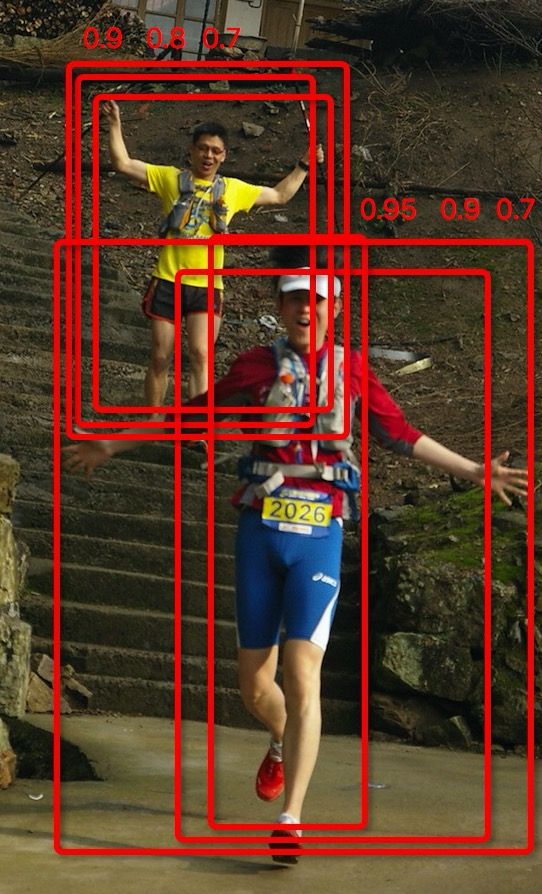
如上图所示，一共有6个识别为人的框，每一个框有一个置信率。
现在需要消除多余的:

· 按置信率排序: 0.95, 0.9, 0.9, 0.8, 0.7, 0.7

· 取最大0.95的框为一个物体框

· 剩余5个框中，去掉与0.95框重叠率IoU大于0.6(可以另行设置)，则保留0.9, 0.8, 0.7三个框

· 重复上面的步骤，直到没有框了，0.9为一个框

· 选出来的为: 0.95, 0.9

所以，整个过程，可以用下图形象的表示出来

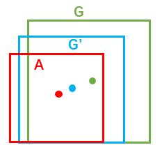
其中，红色的A框是生成的anchor box,而蓝色的G’框就是经过RPN网络训练后得到的较精确的预测框，绿色的G是ground truth box

Bounding box regression

R-CNN中的bounding box回归

下面先介绍R-CNN和Fast R-CNN中所用到的边框回归方法.

(1) 为什么要做Bounding-box regression？

如上图所示，绿色的框为飞机的Ground Truth，红色的框是提取的Region Proposal.那么即便红色的框被分类器识别为飞机，但是由于红色的框定位不准(IoU<0.5)，那么这张图相当于没有正确的检测出飞机.如果我们能对红色的框进行微调，使得经过微调后的窗口跟Ground Truth更接近，这样岂不是定位会更准确.确实，Bounding-box regression 就是用来微调这个窗口的.

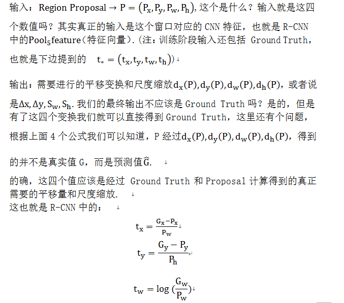
(2) 回归/微调的对象是什么？

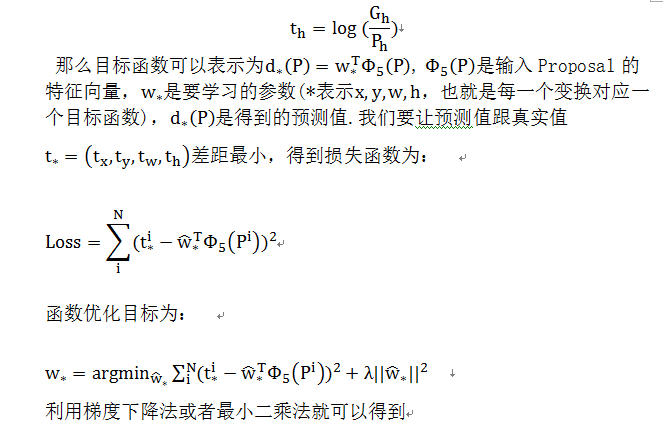
(4) Bounding-box regression（边框回归）
那么经过何种变换才能从图11中的窗口P变为窗口呢？比较简单的思路就是：

注意：只有当Proposal和Ground Truth比较接近时（线性问题），我们才能将其作为训练样本训练我们的线性回归模型，否则会导致训练的回归模型不work（当Proposal跟GT离得较远，就是复杂的非线性问题了，此时用线性回归建模显然不合理）.这个也是G-CNN: an Iterative Grid Based Object Detector多次迭代实现目标准确定位的关键.
线性回归就是给定输入的特征向量X，学习一组参数W，使得经过线性回归后的值跟真实值Y(Ground Truth)非常接近.即.那么Bounding-box中我们的输入以及输出分别是什么呢？

---

代码解读

代码结构图

Faster-RCNN网络结构图如下所示，理解该图对理解整个流程极为重要:

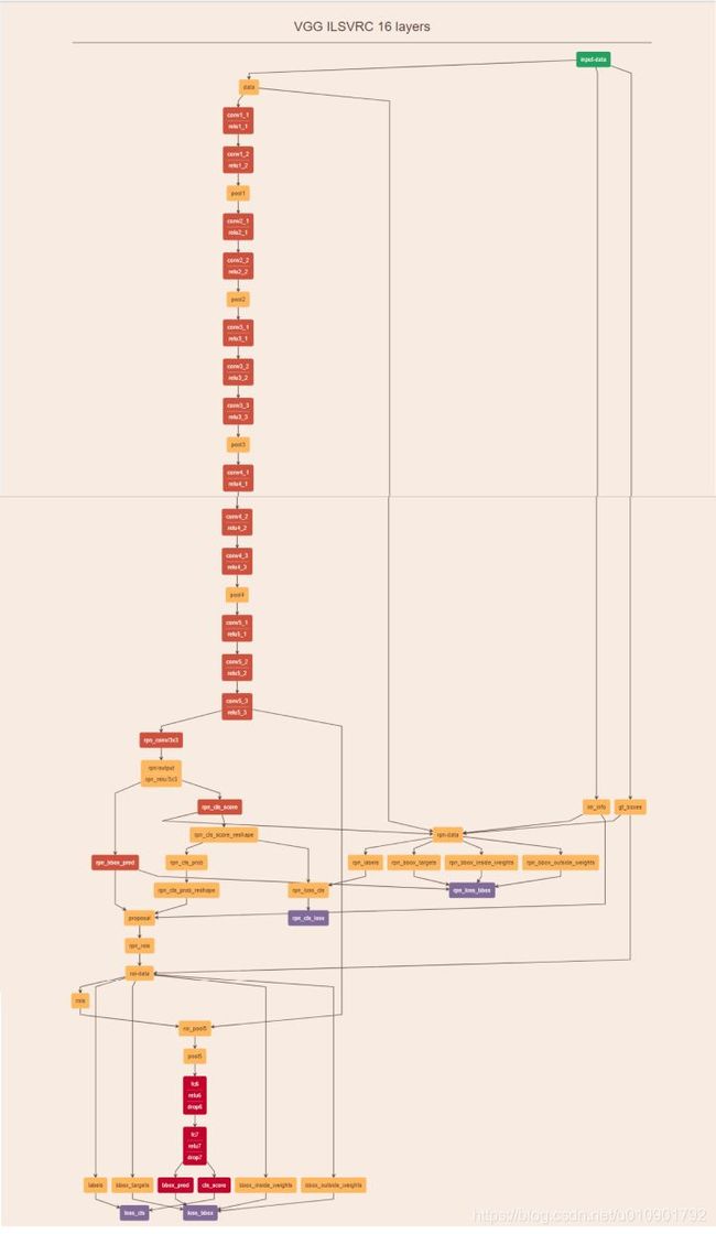
再结合这幅网络结构说明图，可以看的更加清楚：

可以看到，经过了基础网络部分之后得到的 feature map，然后被分为两支，进而得到 proposal，最后通过ROI层得到固定大小的feature，最终进行分类。

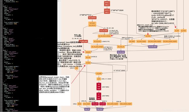
为了更加具体的了解网络的前馈以及训练过程，我把该图的前面抽取特征的基础网络部分略去，把后面部分每个节点的计算以及数据维度做了一个标注，图片如下：

为了更好理解代码结构，可查看代码的结构图：

其详细解释如下：

数据准备

首先，trainval_net.py

imdb, roidb = combined_roidb(args.imdb_name) # 输入参数 imdb_name,默认是 voc_2007_trainval(数据集名字)
print '{:d} roidb entries'.format(len(roidb))

combined_roidb:

 def get_roidb(imdb_name):
    # factory.py 中的函数，调用的是 pascal_voc 的数据集对象
    # get_imdb 默认返回的是 pascal_voc('trainval', '2007')
    # 设置imdb的一些属性，如图片路径，图片名称索引等，未读取真正的图片数据
    imdb = get_imdb(imdb_name)
    print('Loaded dataset `{:s}` for training'.format(imdb.name))
    # 设置proposal方法
    imdb.set_proposal_method(cfg.TRAIN.PROPOSAL_METHOD)
    print('Set proposal method: {:s}'.format(cfg.TRAIN.PROPOSAL_METHOD))
    # 得到用于训练的roidb,定义在train.py,进行了水平翻转，以及为原始roidb添加了一些说明性的属性
    roidb = get_training_roidb(imdb)
    return roidb

  # imdb_names.split('+') 默认值是 voc_2007_trainval
  # 需要调用内部函数 get_roidb
  #如果需要训练多个数据集，就在数据集之间用+号连接
  roidbs = [get_roidb(s) for s in imdb_names.split('+')]
  roidb = roidbs[0]
  if len(roidbs) > 1:#跳过
    for r in roidbs[1:]:
      roidb.extend(r)
    tmp = get_imdb(imdb_names.split('+')[1])
    imdb = datasets.imdb.imdb(imdb_names, tmp.classes)
  else:
    # get_imdb方法定义在dataset/factory.py,通过名字得到imdb
    imdb = get_imdb(imdb_names)# 即前面提到的 imdb=pascal_voc('trainval', '2007')
  return imdb, roidb#roidb应该是属于imdb的.roidb是没有真正的读取数据的，只是建立相关的数据信息

get_roidb

所以我们要先看imdb是如何产生的，然后看如何借助imdb产生roidb

def get_imdb(name):  
    """Get an imdb (image database) by name."""  
    if not __sets.has_key(name):  
        raise KeyError('Unknown dataset: {}'.format(name))  
    return __sets[name]()  

从上面可见，get_imdb这个函数的实现原理：_sets是一个字典，字典的key是数据集的名称，字典的value是一个lambda表达式（即一个函数指针），

__sets[name]()

这句话实际上是调用函数，返回数据集imdb，下面看这个函数：

for year in ['2007', '2012']:
    for split in ['train', 'val', 'trainval', 'test']:
        name = 'voc_{}_{}'.format(year, split)
        __sets[name] = (lambda split=split, year=year: pascal_voc(split, year))

所以可以看到，执行的实际上是pascal_voc函数，参数是split 和 year（ps：默认情况下，name是voc_2007_trainval，所以这里对应的split和year分别是trainval和2007）；
很明显，pascal_voc是一个类，这是调用了该类的构造函数，返回的也是该类的一个实例，所以这下我们清楚了imdb实际上就是pascal_voc的一个实例；

pascal_voc

那么我们来看这个类的构造函数是如何的，以及输入的图片数据在里面是如何组织的：

该类的构造函数如下：基本上就是设置了imdb的一些属性，比如图片的路径，图片名称的索引，并没有把真实的图片数据放进来

class pascal_voc(imdb):
    def __init__(self, image_set, year, devkit_path=None):
        imdb.__init__(self, 'voc_' + year + '_' + image_set)
        self._year = year # 设置年，2007
        self._image_set = image_set # trainval
        self._devkit_path = self._get_default_path() if devkit_path is None \
                            else devkit_path # 数据集的路径'/home/sloan/py-faster-rcnn-master/data/VOCdevkit2007'
        self._data_path = os.path.join(self._devkit_path, 'VOC' + self._year) # '/home/sloan/py-faster-rcnn-master/data/VOCdevkit2007/VOC2007'
        self._classes = ('__background__', # always index 0
                         'aeroplane', 'bicycle', 'bird', 'boat',
                         'bottle', 'bus', 'car', 'cat', 'chair',
                         'cow', 'diningtable', 'dog', 'horse',
                         'motorbike', 'person', 'pottedplant',
                         'sheep', 'sofa', 'train', 'tvmonitor') # 21个类别
        self._class_to_ind = dict(zip(self.classes, xrange(self.num_classes))) #给每个类别赋予一个对应的整数
        self._image_ext = '.jpg' # 图片的扩展名
        self._image_index = self._load_image_set_index() # 把所有图片的名称加载，放在list中，便于索引读取图片
        # Default to roidb handler
        self._roidb_handler = self.selective_search_roidb
        self._salt = str(uuid.uuid4())
        self._comp_id = 'comp4'
 
        # PASCAL specific config options
        self.config = {'cleanup'     : True,
                       'use_salt'    : True,
                       'use_diff'    : False,
                       'matlab_eval' : False,
                       'rpn_file'    : None,
                       'min_size'    : 2}
        # 这两句就是检查前面的路径是否存在合法了，否则后面无法运行
        assert os.path.exists(self._devkit_path), \
                'VOCdevkit path does not exist: {}'.format(self._devkit_path)
        assert os.path.exists(self._data_path), \
                'Path does not exist: {}'.format(self._data_path)

#
class imdb(object):
    """Image database."""

    def __init__(self, name):
        self._name = name
        self._num_classes = 0
        self._classes = []
        self._image_index = []
        self._obj_proposer = 'selective_search'
        self._roidb = None
        self._roidb_handler = self.default_roidb
        # Use this dict for storing dataset specific config options
        self.config = {}

注：如果想训练自己的数据，把self._classes的内容换成自己的类别, '_background_'要保留。

得到的 imdb = pascal_voc(‘trainval’, ‘2007’) 记录的内容如下：

[1] - _class_to_ind，dict 类型，key 是类别名，value 是 label 值(从 0 开始)，其中 (key[0], value[0]) = [background, 0]

[2] - _classes，object 类别名，共 20(object classes) + 1(background) = 21 classes.

[3] - _data_path，数据集路径

[4] - _image_ext，’.jpg’ 数据类型

[5] - _image_index，图片索引列表

[6] - _image_set，’trainval’

[7] - _name，数据集名称 voc_2007_trainval

[8] - _num_classes，0

[9] - _obj_proposer，selective_search

[10] - _roidb，None

[11] - classes，与_classes 相同

[12] - image_index，与_image_index 相同

[13] - name，数据集名称，与 _name 相同

[14] - num_classes，类别数，21

[15] - num_images，图片数

[16] - config，dict 类型，PASCAL 数据集指定的配置

set_proposal_method

那么有了imdb之后，roidb又有什么不同呢？为什么实际输入的数据是roidb呢？

前面我们已经得到了imdb，但是imdb的成员roidb还是空白，啥都没有，那么roidb是如何生成的，其中又包含了哪些信息呢？

imdb.set_proposal_method(cfg.TRAIN.PROPOSAL_METHOD)

上面调用的函数，为imdb添加了roidb的数据，我们看看如何添加的，见下面这个函数：

    def set_proposal_method(self, method):
        method = eval('self.' + method + '_roidb')
        self.roidb_handler = method

这里method传入的是一个str：gt，所以method=eval(‘self.gt_roidb’)

gt_roidb

第一次加载数据时放到缓存里，之后就直接到缓存取数据即可。

  def gt_roidb(self):
    """
    Return the database of ground-truth regions of interest.

    This function loads/saves from/to a cache file to speed up future calls.
    """
    cache_file = os.path.join(self.cache_path, self.name + '_gt_roidb.pkl')
    if os.path.exists(cache_file):
      with open(cache_file, 'rb') as fid:
        try:
          roidb = pickle.load(fid)
        except:
          roidb = pickle.load(fid, encoding='bytes')
      print('{} gt roidb loaded from {}'.format(self.name, cache_file))
      return roidb

    gt_roidb = [self._load_pascal_annotation(index)
                for index in self.image_index]
    with open(cache_file, 'wb') as fid:
      pickle.dump(gt_roidb, fid, pickle.HIGHEST_PROTOCOL)
    print('wrote gt roidb to {}'.format(cache_file))

    return gt_roidb

get_training_roidb

有了roidb后，后面的get_training_roidb(imdb)完成什么功能：将roidb中的元素由5011个，通过水平对称变成10022个；将index这个list的元素相应的也翻一番；

def get_training_roidb(imdb):
  """Returns a roidb (Region of Interest database) for use in training."""
  if cfg.TRAIN.USE_FLIPPED:# 是否进行图片翻转
    print('Appending horizontally-flipped training examples...')
    # 对imdb中涉及到的图像做了一个水平镜像，使得trainval中的5011张图片，变成了10022张图片；
    imdb.append_flipped_images()
    print('done')

  print('Preparing training data...')
  # # 为原始数据集的roidb添加一些说明性的属性，max-overlap,max-classes...
  rdl_roidb.prepare_roidb(imdb)# 准备数据
  print('done')

  return imdb.roidb

append_flipped_images

首先我们看看append_flipped_images函数：可以发现，roidb是imdb的一个成员变量，roidb是一个list（每个元素对应一张图片），list中的元素是一个字典，字典中存放了5个key，分别是boxes信息，每个box的class信息，是否是flipped的标志位，重叠信息gt_overlaps，以及seg_areas；分析该函数可知，将box的值按照水平对称，原先roidb中只有5011个元素，经过水平对称后通过append增加到5011*2=10022个；

  def append_flipped_images(self):
    num_images = self.num_images
    widths = self._get_widths()
    for i in range(num_images):
      boxes = self.roidb[i]['boxes'].copy()
      oldx1 = boxes[:, 0].copy()
      oldx2 = boxes[:, 2].copy()
      boxes[:, 0] = widths[i] - oldx2 - 1
      boxes[:, 2] = widths[i] - oldx1 - 1
      assert (boxes[:, 2] >= boxes[:, 0]).all()
      entry = {'boxes': boxes,
               'gt_overlaps': self.roidb[i]['gt_overlaps'],
               'gt_classes': self.roidb[i]['gt_classes'],
               'flipped': True}
      self.roidb.append(entry)
    self._image_index = self._image_index * 2

prepare_roidb

def prepare_roidb(imdb):
  """Enrich the imdb's roidb by adding some derived quantities that
  are useful for training. This function precomputes the maximum
  overlap, taken over ground-truth boxes, between each ROI and
  each ground-truth box. The class with maximum overlap is also
  recorded.
  """
  roidb = imdb.roidb
  if not (imdb.name.startswith('coco')):
    sizes = [PIL.Image.open(imdb.image_path_at(i)).size
         for i in range(imdb.num_images)]
  for i in range(len(imdb.image_index)):
    roidb[i]['image'] = imdb.image_path_at(i)#图片名
    if not (imdb.name.startswith('coco')):
      roidb[i]['width'] = sizes[i][0]#图片width
      roidb[i]['height'] = sizes[i][1]#图片height
    # need gt_overlaps as a dense array for argmax
    gt_overlaps = roidb[i]['gt_overlaps'].toarray()#转换成one_hot
    # max overlap with gt over classes (columns)
    max_overlaps = gt_overlaps.max(axis=1)
    # gt class that had the max overlap
    max_classes = gt_overlaps.argmax(axis=1)
    roidb[i]['max_classes'] = max_classes
    roidb[i]['max_overlaps'] = max_overlaps
    # sanity checks 合理性检查
    # max overlap of 0 => class should be zero (background)
    zero_inds = np.where(max_overlaps == 0)[0]
    assert all(max_classes[zero_inds] == 0)
    # max overlap > 0 => class should not be zero (must be a fg class)
    nonzero_inds = np.where(max_overlaps > 0)[0]
    assert all(max_classes[nonzero_inds] != 0)

train_net

roidb 应该是属于 imdb 的.

roidb 是没有真正的读取数据的，只是建立相关的数据信息.

def train_net(network, imdb, roidb, valroidb, output_dir, tb_dir,
              pretrained_model=None,
              max_iters=40000):
  """Train a Faster R-CNN network."""
  #这里对 roidb 先进行处理，即函数 filter_roidb，去除没用的 RoIs
  roidb = filter_roidb(roidb)
  valroidb = filter_roidb(valroidb)

  tfconfig = tf.ConfigProto(allow_soft_placement=True)
  tfconfig.gpu_options.allow_growth = True

  with tf.Session(config=tfconfig) as sess:
    sw = SolverWrapper(sess, network, imdb, roidb, valroidb, output_dir, tb_dir,
                       pretrained_model=pretrained_model)
    print('Solving...')
    sw.train_model(sess, max_iters)
    print('done solving')

filter_roidb

这里对 roidb 先进行处理，即函数 filter_roidb，去除没用的 RoIs，

def filter_roidb(roidb):
  """Remove roidb entries that have no usable RoIs."""

  # 删掉没用的RoIs, 有效的图片必须各有前景和背景ROI
  def is_valid(entry):
    # Valid images have:
    #   (1) At least one foreground RoI OR
    #   (2) At least one background RoI
    overlaps = entry['max_overlaps']
    # find boxes with sufficient overlap
    fg_inds = np.where(overlaps >= cfg.TRAIN.FG_THRESH)[0]
    # Select background RoIs as those within [BG_THRESH_LO, BG_THRESH_HI)
    bg_inds = np.where((overlaps < cfg.TRAIN.BG_THRESH_HI) &
                       (overlaps >= cfg.TRAIN.BG_THRESH_LO))[0]
    # image is only valid if such boxes exist
    valid = len(fg_inds) > 0 or len(bg_inds) > 0
    return valid

  num = len(roidb)
  filtered_roidb = [entry for entry in roidb if is_valid(entry)]
  num_after = len(filtered_roidb)
  print('Filtered {} roidb entries: {} -> {}'.format(num - num_after,
                                                     num, num_after))
  return filtered_roidb

RoIDataLayer

目前为止，上面只是准备了roidb的相关信息而已，真正的数据处理操作是在类RoIDataLayer里，

def forward(self, bottom, top):函数中开始的，这个类在lib/roi_data_layer/layer.py文件中

blobs = self._get_next_minibatch()这句话产生了我们需要的数据blobs；这个函数又调用了minibatch.py文件中的def get_minibatch(roidb, num_classes):函数；

然后又调用了def _get_image_blob(roidb, scale_inds):函数；在这个函数中，我们终于发现了cv2.imread函数，也就是最终的读取图片到内存的地方：

def _get_image_blob(roidb, scale_inds):
  """Builds an input blob from the images in the roidb at the specified
  scales.
  """
  num_images = len(roidb)
  processed_ims = []
  im_scales = []
  for i in range(num_images):
    im = cv2.imread(roidb[i]['image'])
    if roidb[i]['flipped']:
      im = im[:, ::-1, :]
    target_size = cfg.TRAIN.SCALES[scale_inds[i]]
    im, im_scale = prep_im_for_blob(im, cfg.PIXEL_MEANS, target_size,
                    cfg.TRAIN.MAX_SIZE)
    im_scales.append(im_scale)
    processed_ims.append(im)

  # Create a blob to hold the input images
  blob = im_list_to_blob(processed_ims)

  return blob, im_scales

终于，数据准备完事…

训练阶段

SolverWrapper通过construct_graph创建网络、train_op等。

construct_graph通过Network的create_architecture创建网络。

注：在代码中，anchor,proposal,rois,boxes代表的含义其实都是一样的，都是推荐的区域或者框，不过有所区别的地方在于
这几个名词有一个递进的关系，最开始的使锚定的框anchor,数量最多约为2万个(根据resize后的图片大小不同数量有所变化)
然后是rpn网络推荐的框proposal,数量较多，train时候有2000个，
再然后是实际分类时候用到的rois框，每张图片有256个，
最后得到的结果就是boxes

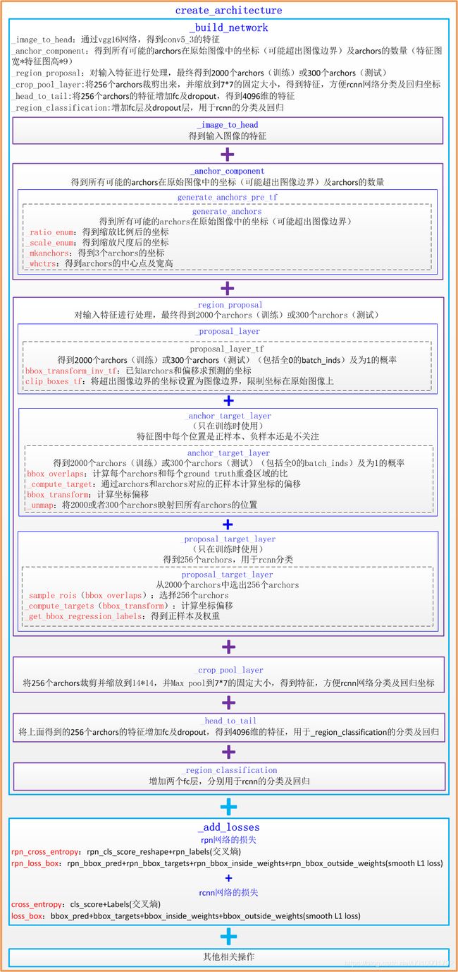
create_architecture

create_architecture通过_build_network具体创建网络模型、损失及其他相关操作，得到rois, cls_prob, bbox_pred，定义如下

 def create_architecture(self, mode, num_classes, tag=None,
                          anchor_scales=(8, 16, 32), anchor_ratios=(0.5, 1, 2)):
    self._image = tf.placeholder(tf.float32, shape=[1, None, None, 3])
    #图像信息，高、宽、缩放比例im_scales（压缩到最小边长为600，但是如果压缩之后最大边长超过2000，则以最大边长2000为限制条件）
    #原图大小(720*1280),resize后图像大小为(600*1067). im_scales=600/720=0.8333
    self._im_info = tf.placeholder(tf.float32, shape=[3])#
    self._gt_boxes = tf.placeholder(tf.float32, shape=[None, 5])
    self._tag = tag

    self._num_classes = num_classes
    self._mode = mode
    self._anchor_scales = anchor_scales
    self._num_scales = len(anchor_scales)

    self._anchor_ratios = anchor_ratios
    self._num_ratios = len(anchor_ratios)

    self._num_anchors = self._num_scales * self._num_ratios

    training = mode == 'TRAIN'
    testing = mode == 'TEST'

    assert tag != None

    # handle most of the regularizers here
    weights_regularizer = tf.contrib.layers.l2_regularizer(cfg.TRAIN.WEIGHT_DECAY)
    if cfg.TRAIN.BIAS_DECAY:
      biases_regularizer = weights_regularizer
    else:
      biases_regularizer = tf.no_regularizer

    # list as many types of layers as possible, even if they are not used now
    with arg_scope([slim.conv2d, slim.conv2d_in_plane, \
                    slim.conv2d_transpose, slim.separable_conv2d, slim.fully_connected], 
                    weights_regularizer=weights_regularizer,
                    biases_regularizer=biases_regularizer, 
                    biases_initializer=tf.constant_initializer(0.0)):
      #rois:256个anchors的类别(训练时为每个anchors的类别，测试时全0)
      #cls_prob:256个anchors每一类别的概率
      #bbox_pred:预测位置信息的偏移
      rois, cls_prob, bbox_pred = self._build_network(training)#用于创建网络

    layers_to_output = {'rois': rois}

    for var in tf.trainable_variables():
      self._train_summaries.append(var)

    if testing:
      stds = np.tile(np.array(cfg.TRAIN.BBOX_NORMALIZE_STDS), (self._num_classes))
      means = np.tile(np.array(cfg.TRAIN.BBOX_NORMALIZE_MEANS), (self._num_classes))
      self._predictions["bbox_pred"] *= stds#训练时_region_proposal中预测的位置偏移减均值除标准差，因而测试时需要反过来
      self._predictions["bbox_pred"] += means
    else:
      self._add_losses()
      layers_to_output.update(self._losses)

      val_summaries = []
      with tf.device("/cpu:0"):
        val_summaries.append(self._add_gt_image_summary())
        for key, var in self._event_summaries.items():
          val_summaries.append(tf.summary.scalar(key, var))
        for key, var in self._score_summaries.items():
          self._add_score_summary(key, var)
        for var in self._act_summaries:
          self._add_act_summary(var)
        for var in self._train_summaries:
          self._add_train_summary(var)

      self._summary_op = tf.summary.merge_all()
      self._summary_op_val = tf.summary.merge(val_summaries)

    layers_to_output.update(self._predictions)

    return layers_to_output

_build_network

_build_netword用于创建网络

总体流程：网络通过vgg1-5得到特征net_conv后，送入rpn网络得到候选区域anchors，去除超出图像边界的anchors并选出2000个anchors用于训练rpn网络（300个用于测试）。并进一步选择256个anchors（用于rcnn分类）。之后将这256个anchors的特征根据rois进行裁剪缩放及pooling，得到相同大小7*7的特征pool5，pool5通过两个fc层得到4096维特征fc7，fc7送入_region_classification（2个并列的fc层），得到21维的cls_score和21*4维的bbox_pred。

def _build_network(self, is_training=True):
  # select initializers
  if cfg.TRAIN.TRUNCATED:
    initializer = tf.truncated_normal_initializer(mean=0.0, stddev=0.01)
    initializer_bbox = tf.truncated_normal_initializer(mean=0.0, stddev=0.001)
  else:
    initializer = tf.random_normal_initializer(mean=0.0, stddev=0.01)
    initializer_bbox = tf.random_normal_initializer(mean=0.0, stddev=0.001)

  net_conv = self._image_to_head(is_training)#得到输入图像的特征
  with tf.variable_scope(self._scope, self._scope):
    # build the anchors for the image
    #生成anchors，得到所有可能的anchors在原始图像中的坐标（可能超出图像边界）及anchors的数量
    self._anchor_component()
    # region proposal network
    #RPN网络，得到256个anchors的类别(训练时为每个anchors的类别，测试时全0)及位置(后四维)
    rois = self._region_proposal(net_conv, is_training, initializer)
    # region of interest pooling
    #ROI pooling
    if cfg.POOLING_MODE == 'crop':
      pool5 = self._crop_pool_layer(net_conv, rois, "pool5")#对特征图通过rois得到候选区域，并对候选区域进行缩放，得到14*14的固定大小，进一步pooling成7*7大小
    else:
      raise NotImplementedError

  fc7 = self._head_to_tail(pool5, is_training)#对固定大小的rois增加fc及dropout,得到4096维的特征，用于分类及回归
  with tf.variable_scope(self._scope, self._scope):
    # region classification
    #分类/回归网络，对rois进行分类，完成目标检测；进行回归，得到预测坐标
    cls_prob, bbox_pred = self._region_classification(fc7, is_training, 
                                                      initializer, initializer_bbox)

  self._score_summaries.update(self._predictions)

  #rois:256*5
  #cls_prob:256*21(类别数)
  #bbox_pred:256*84(类别数*4)
  return rois, cls_prob, bbox_pred

_image_to_head

_image_to_head用于得到输入图像的特征

该函数位于vgg16.py中，定义如下

def _image_to_head(self, is_training, reuse=None):
  with tf.variable_scope(self._scope, self._scope, reuse=reuse):
    net = slim.repeat(self._image, 2, slim.conv2d, 64, [3, 3],
                        trainable=False, scope='conv1')
    net = slim.max_pool2d(net, [2, 2], padding='SAME', scope='pool1')
    net = slim.repeat(net, 2, slim.conv2d, 128, [3, 3],
                      trainable=False, scope='conv2')
    net = slim.max_pool2d(net, [2, 2], padding='SAME', scope='pool2')
    net = slim.repeat(net, 3, slim.conv2d, 256, [3, 3],
                      trainable=is_training, scope='conv3')
    net = slim.max_pool2d(net, [2, 2], padding='SAME', scope='pool3')
    net = slim.repeat(net, 3, slim.conv2d, 512, [3, 3],
                      trainable=is_training, scope='conv4')
    net = slim.max_pool2d(net, [2, 2], padding='SAME', scope='pool4')
    net = slim.repeat(net, 3, slim.conv2d, 512, [3, 3],
                      trainable=is_training, scope='conv5')

  self._act_summaries.append(net)
  self._layers['head'] = net
  
  return net

_anchor_component

_anchor_component：用于得到所有可能的anchors在原始图像中的坐标（可能超出图像边界）及anchors的数量（特征图宽*特征图高*9）。该函数使用的self._im_info，为一个3维向量，[0]代表图像宽，[1]代表图像高，[2]代表图像缩放的比例（将图像宽缩放到600，或高缩放到1000的最小比例，比如缩放到600*900、850*1000）。该函数调用generate_anchors_pre_tf并进一步调用generate_anchors来得到所有可能的anchors在原始图像中的坐标及anchors的个数（由于图像大小不一样，因而最终anchor的个数也不一样）。
generate_anchors_pre_tf步骤如下：

1. 通过_ratio_enum得到anchor时，使用 (0, 0, 15, 15) 的基准窗口，先通过ratio=[0.5,1,2]的比例得到anchors。ratio指的是像素总数（宽*高）的比例，而不是宽或者高的比例，得到如下三个archor（每个archor为左上角和右下角的坐标）：

2. 而后在通过scales=(8, 16, 32)得到放大倍数后的anchors。scales时，将上面的每个都直接放大对应的倍数，最终得到9个anchors（每个anchor为左上角和右下角的坐标）。将上面三个anchors分别放大就行了，因而本文未给出该图。

之后通过tf.add(anchor_constant, shifts)得到缩放后的每个点的9个anchor在原始图的矩形框。anchor_constant：1*9*4。shifts：N*1*4。N为缩放后特征图的像素数。将维度从N*9*4变换到(N*9)*4，得到缩放后的图像每个点在原始图像中的anchors。

  def _anchor_component(self):
    with tf.variable_scope('ANCHOR_' + self._tag) as scope:
      # just to get the shape right
      #tf.ceil 向上取整
      height = tf.to_int32(tf.ceil(self._im_info[0] / np.float32(self._feat_stride[0])))#图像经过VGG16得到特征图的高宽
      width = tf.to_int32(tf.ceil(self._im_info[1] / np.float32(self._feat_stride[0])))
      if cfg.USE_E2E_TF:
        #通过特征图宽高，_feat_stride（特征图对原始图缩小的比例）等得到图像上的所有可能的anchors(坐标可能超出原始图像边界)和anchor数量
        anchors, anchor_length = generate_anchors_pre_tf(
          height,
          width,
          self._feat_stride,
          self._anchor_scales,
          self._anchor_ratios#指的是像素总数(宽*高)的比例
        )
      else:
        anchors, anchor_length = tf.py_func(generate_anchors_pre,#得到所有可能的anchors在原始图像中的坐标(可能超出图像边界)及anchors数量
                                            [height, width,
                                             self._feat_stride, self._anchor_scales, self._anchor_ratios],
                                            [tf.float32, tf.int32], name="generate_anchors")
      anchors.set_shape([None, 4])
      anchor_length.set_shape([])
      self._anchors = anchors
      self._anchor_length = anchor_length

generate_anchors_pre

def generate_anchors_pre_tf(height, width, feat_stride=16, anchor_scales=(8, 16, 32), anchor_ratios=(0.5, 1, 2)):
  shift_x = tf.range(width) * feat_stride # 得到所有anchors在原始图像的起始x坐标：(0,feat_stride,2*feat_stride,...)
  shift_y = tf.range(height) * feat_stride # 得到所有anchors在原始图像的起始y坐标：(0,feat_stride,2*feat_stride,...)
  shift_x, shift_y = tf.meshgrid(shift_x, shift_y)
  sx = tf.reshape(shift_x, shape=(-1,))
  sy = tf.reshape(shift_y, shape=(-1,))
  shifts = tf.transpose(tf.stack([sx, sy, sx, sy]))#width*height个四位矩阵
  K = tf.multiply(width, height)#特征图总共像素数
  shifts = tf.transpose(tf.reshape(shifts, shape=[1, K, 4]), perm=(1, 0, 2))#增加一维，变成1*(width*height)*4矩阵，而后变换纬度为(width*height)*1*4
  #得到9个anchors在原始图像中的四个坐标(放大比例默认为16)
  anchors = generate_anchors(ratios=np.array(anchor_ratios), scales=np.array(anchor_scales))
  A = anchors.shape[0]#9
  anchor_constant = tf.constant(anchors.reshape((1, A, 4)), dtype=tf.int32)#增加维度为1*9*4

  length = K * A#总共的anchors的个数(每个点对应A=9个anchor,共K=height*width个点)
  #1*9*4的base anchor和(width*height)*1*4的偏移矩阵进行broadcast相加，得到(width*height)*9*4,
  #并改变形状为(width*height*9)*4,得到所有的anchors的四个坐标
  anchors_tf = tf.reshape(tf.add(anchor_constant, shifts), shape=(length, 4))
  
  return tf.cast(anchors_tf, dtype=tf.float32), length

generate_anchors

def generate_anchors(base_size=16, ratios=[0.5, 1, 2],
                     scales=2 ** np.arange(3, 6)):
  """
  Generate anchor (reference) windows by enumerating aspect ratios X
  scales wrt a reference (0, 0, 15, 15) window.
  """

  base_anchor = np.array([1, 1, base_size, base_size]) - 1#base_anchor的四个坐标
  ratio_anchors = _ratio_enum(base_anchor, ratios)#通过ratio得到3个anchors的坐标(3*4)
  anchors = np.vstack([_scale_enum(ratio_anchors[i, :], scales)#3*4矩阵变成9*4矩阵，得到9个anchors的坐标
                       for i in range(ratio_anchors.shape[0])])
  return anchors


def _whctrs(anchor):
  """
  Return width, height, x center, and y center for an anchor (window).
  """

  w = anchor[2] - anchor[0] + 1#宽
  h = anchor[3] - anchor[1] + 1#高
  x_ctr = anchor[0] + 0.5 * (w - 1)#中心x
  y_ctr = anchor[1] + 0.5 * (h - 1)#中心y
  return w, h, x_ctr, y_ctr


def _mkanchors(ws, hs, x_ctr, y_ctr):
  """
  Given a vector of widths (ws) and heights (hs) around a center
  (x_ctr, y_ctr), output a set of anchors (windows).
  """

  ws = ws[:, np.newaxis]#3维向量变成3*1矩阵
  hs = hs[:, np.newaxis]
  anchors = np.hstack((x_ctr - 0.5 * (ws - 1),#3*4矩阵
                       y_ctr - 0.5 * (hs - 1),
                       x_ctr + 0.5 * (ws - 1),
                       y_ctr + 0.5 * (hs - 1)))
  return anchors


def _ratio_enum(anchor, ratios):#缩放比例为像素总数的比例，而非单独宽或者高的比例
  """
  Enumerate a set of anchors for each aspect ratio wrt an anchor.
  """

  w, h, x_ctr, y_ctr = _whctrs(anchor)#得到中心位置和宽高 [16,16,7.5,7.5]
  size = w * h#总共像素数 256
  size_ratios = size / ratios#缩放比例 [512,256,128]
  ws = np.round(np.sqrt(size_ratios))#缩放后的宽，3维向量，值由大到小[23,16,11]
  hs = np.round(ws * ratios)#缩放后的高，值由小到大 [12,16,22]
  anchors = _mkanchors(ws, hs, x_ctr, y_ctr)#根据中心及宽高得到3个anchors的四个坐标
  return anchors


def _scale_enum(anchor, scales):
  """
  Enumerate a set of anchors for each scale wrt an anchor.
  """

  w, h, x_ctr, y_ctr = _whctrs(anchor)
  ws = w * scales
  hs = h * scales
  anchors = _mkanchors(ws, hs, x_ctr, y_ctr)
  return anchors

_region_proposal

_region_proposal用于将vgg16的conv5的特征通过3*3的滑动窗得到rpn特征，进行两条并行的线路，分别送入cls和reg网络。

cls网络判断通过1*1的卷积得到anchors是正样本还是负样本（由于anchors过多，还有可能有不关心的anchors，使用时只使用正样本和负样本），用于二分类rpn_cls_score；

reg网络对通过1*1的卷积回归出anchors的坐标偏移rpn_bbox_pred。这两个网络共用3*3 conv（rpn）。由于每个位置有k个anchor，因而每个位置均有2k个soores和4k个coordinates。

cls（将输入的512维降低到2k维）：3*3 conv + 1*1 conv（2k个scores，k为每个位置archors个数，如9）

在第一次使用_reshape_layer时，由于输入bottom为1*？*？*2k，先得到caffe中的数据顺序（tf为batchsize*height*width*channels，caffe中为batchsize*channels*height*width）to_caffe：1*2k*？*？，而后reshape后得到reshaped为1*2*？*？，最后在转回tf的顺序to_tf为1*？*？*2，得到rpn_cls_score_reshape。之后通过rpn_cls_prob_reshape（softmax的值，只针对最后一维，即2计算softmax），得到概率rpn_cls_prob_reshape（其最大值，即为预测值rpn_cls_pred），再次_reshape_layer，得到1*？*？*2k的rpn_cls_prob，为原始的概率。

reg（将输入的512维降低到4k维）：3*3 conv + 1*1 conv（4k个coordinates，k为每个位置archors个数，如9）。

_region_proposal定义如下：

 def _region_proposal(self, net_conv, is_training, initializer):
    #vgg16提取后的特征图，先进行3*3卷积
    #3*3的conv,作为rpn网络
    rpn = slim.conv2d(net_conv, cfg.RPN_CHANNELS, [3, 3], trainable=is_training, weights_initializer=initializer,
                        scope="rpn_conv/3x3")
    self._act_summaries.append(rpn)
    #每个框进行2分类，判断前景还是背景
    #1*1的conv,得到每个位置的9个anchors分类特征[1,?,?,9*2],
    rpn_cls_score = slim.conv2d(rpn, self._num_anchors * 2, [1, 1], trainable=is_training,
                                weights_initializer=initializer,
                                padding='VALID', activation_fn=None, scope='rpn_cls_score')
    # change it so that the score has 2 as its channel size
    #reshape成标准形式
    #[1,?,?,9*2]-->[1,?*9.?,2]
    rpn_cls_score_reshape = self._reshape_layer(rpn_cls_score, 2, 'rpn_cls_score_reshape')
    #以最后一维为特征长度，得到所有特征的概率[1,?*9.?,2]
    rpn_cls_prob_reshape = self._softmax_layer(rpn_cls_score_reshape, "rpn_cls_prob_reshape")
    #得到每个位置的9个anchors预测的类别，[1,?,9,?]的列向量
    rpn_cls_pred = tf.argmax(tf.reshape(rpn_cls_score_reshape, [-1, 2]), axis=1, name="rpn_cls_pred")
    #变换回原始纬度，[1,?*9.?,2]-->[1,?,?,9*2]
    rpn_cls_prob = self._reshape_layer(rpn_cls_prob_reshape, self._num_anchors * 2, "rpn_cls_prob")
    #1*1的conv,每个位置的9个anchors回归位置偏移[1,?,?,9*4]
    rpn_bbox_pred = slim.conv2d(rpn, self._num_anchors * 4, [1, 1], trainable=is_training,
                                weights_initializer=initializer,
                                padding='VALID', activation_fn=None, scope='rpn_bbox_pred')
    if is_training:
      #1.使用经过rpn网络层后生成的rpn_cls_prob把anchor位置进行第一次修正
      #2.按照得分排序，取前12000个anchor,再nms,取前面2000个（在test的时候就变成了6000和300）
      rois, roi_scores = self._proposal_layer(rpn_cls_prob, rpn_bbox_pred, "rois")
      #获取属于rpn网络的label:通过对所有的anchor与所有的GT计算IOU，通过消除再图像外部的anchor,计算IOU>=0.7为正样本，IOU<0.3为负样本，
      #得到再理想情况下各自一半的256个正负样本(实际上正样本大多只有10-100个之间，相对负样本偏少)
      rpn_labels = self._anchor_target_layer(rpn_cls_score, "anchor")#rpn_labels:特征图中每个位置对应的正样本、负样本还是不关注
      # Try to have a deterministic order for the computing graph, for reproducibility
      with tf.control_dependencies([rpn_labels]):
        #获得属于最后的分类网络的label
        #因为之前的anchor位置已经修正过了，所以这里又计算了一次经过proposal_layer修正后的box与GT的IOU来得到label
        #但是阈值不一样了，变成了大于等于0.5为1，小于为0，并且这里得到的正样本很少，通常只有2-20个，甚至有0个，
        #并且正样本最多为64个，负样本则有比较多个，相应的也重新计算了一次bbox_targets
        #另外，从RPN网络出来的2000余个rois中挑选256个
        rois, _ = self._proposal_target_layer(rois, roi_scores, "rpn_rois")#通过post_nms_topN个anchors的位置及为1（正样本）的概率得到256个rois及对应信息
    else:
      if cfg.TEST.MODE == 'nms':
        rois, _ = self._proposal_layer(rpn_cls_prob, rpn_bbox_pred, "rois")
      elif cfg.TEST.MODE == 'top':
        rois, _ = self._proposal_top_layer(rpn_cls_prob, rpn_bbox_pred, "rois")
      else:
        raise NotImplementedError

    self._predictions["rpn_cls_score"] = rpn_cls_score#每个位置的9个anchors是正样本还是负样本
    self._predictions["rpn_cls_score_reshape"] = rpn_cls_score_reshape#每个anchors是正样本还是负样本
    self._predictions["rpn_cls_prob"] = rpn_cls_prob#每个位置的9个anchors是正样本和负样本的概率
    self._predictions["rpn_cls_pred"] = rpn_cls_pred#每个位置的9个anchors预测的类别，[1,?,9,?]的列向量
    self._predictions["rpn_bbox_pred"] = rpn_bbox_pred#每个位置的9个anchors回归位置偏移
    self._predictions["rois"] = rois#256个anchors的类别(第一维)及位置(后四维)

    return rois#返回256个anchors的类别(第一维，训练时为每个anchors的类别，测试时全0)及位置(后四维)

_proposal_layer

_proposal_layer调用proposal_layer_tf，通过(N*9)*4个anchors，计算估计后的坐标（bbox_transform_inv_tf），并对坐标进行裁剪（clip_boxes_tf）及非极大值抑制（tf.image.non_max_suppression，可得到符合条件的索引indices）的anchors：rois及这些anchors为正样本的概率：rpn_scores。rois为m*5维，rpn_scores为m*4维，其中m为经过非极大值抑制后得到的候选区域个数（训练时2000个，测试时300个）。m*5的第一列为全为0的batch_inds，后4列为坐标（坐上+右下）

_proposal_layer如下

def _proposal_layer(self, rpn_cls_prob, rpn_bbox_pred, name):
  with tf.variable_scope(name) as scope:
    if cfg.USE_E2E_TF:
      rois, rpn_scores = proposal_layer_tf(
        rpn_cls_prob,
        rpn_bbox_pred,
        self._im_info,
        self._mode,
        self._feat_stride,
        self._anchors,
        self._num_anchors
      )
    else:
      rois, rpn_scores = tf.py_func(proposal_layer,
                            [rpn_cls_prob, rpn_bbox_pred, self._im_info, self._mode,
                             self._feat_stride, self._anchors, self._num_anchors],
                            [tf.float32, tf.float32], name="proposal")

    rois.set_shape([None, 5])
    rpn_scores.set_shape([None, 1])

  return rois, rpn_scores

proposal_layer_tf

def proposal_layer_tf(rpn_cls_prob, rpn_bbox_pred, im_info, cfg_key, _feat_stride, anchors, num_anchors):
  if type(cfg_key) == bytes:
    cfg_key = cfg_key.decode('utf-8')
  pre_nms_topN = cfg[cfg_key].RPN_PRE_NMS_TOP_N
  post_nms_topN = cfg[cfg_key].RPN_POST_NMS_TOP_N#训练时为2000，测试时为300
  nms_thresh = cfg[cfg_key].RPN_NMS_THRESH#nms的阈值，为0.7

  # Get the scores and bounding boxes
  scores = rpn_cls_prob[:, :, :, num_anchors:]#[1,?,?,(9*2)]取后9个，应该是前9个代表9个anchors为背景的概率，后9个代表9个anchors为前景的概率
  scores = tf.reshape(scores, shape=(-1,))
  rpn_bbox_pred = tf.reshape(rpn_bbox_pred, shape=(-1, 4))#所有的anchors的四个坐标

  proposals = bbox_transform_inv_tf(anchors, rpn_bbox_pred)#已知anchors和偏移求预测的坐标
  proposals = clip_boxes_tf(proposals, im_info[:2])#限制预测坐标在原始图像上

  # Non-maximal suppression
  #通过nms得到分支最大的post_num_topN个坐标的索引
  indices = tf.image.non_max_suppression(proposals, scores, max_output_size=post_nms_topN, iou_threshold=nms_thresh)

  boxes = tf.gather(proposals, indices)#得到post_nms_topN个对应的坐标
  boxes = tf.to_float(boxes)
  scores = tf.gather(scores, indices)#得到post_nms_topN个对应的为1的概率
  scores = tf.reshape(scores, shape=(-1, 1))

  # Only support single image as input
  batch_inds = tf.zeros((tf.shape(indices)[0], 1), dtype=tf.float32)
  blob = tf.concat([batch_inds, boxes], 1)#post_nms_topN*1个batch_inds和post_nms_topN*4个坐标concat,得到post_nms_topN*5的blob

  return blob, scores

bbox_transform_inv_tf

已知anchors和偏移求预测的坐标

def bbox_transform_inv_tf(boxes, deltas):
  boxes = tf.cast(boxes, deltas.dtype)
  widths = tf.subtract(boxes[:, 2], boxes[:, 0]) + 1.0#宽
  heights = tf.subtract(boxes[:, 3], boxes[:, 1]) + 1.0#高
  ctr_x = tf.add(boxes[:, 0], widths * 0.5)#中心x
  ctr_y = tf.add(boxes[:, 1], heights * 0.5)#中心y

  dx = deltas[:, 0] #预测的tx
  dy = deltas[:, 1] #预测的ty
  dw = deltas[:, 2] #预测的tw
  dh = deltas[:, 3]#预测的th

  pred_ctr_x = tf.add(tf.multiply(dx, widths), ctr_x)#公式2已知xa,wa,tx反过来求预测的x中心坐标
  pred_ctr_y = tf.add(tf.multiply(dy, heights), ctr_y)#公式2已知ya,ha,ty反过来求预测的y中心坐标
  pred_w = tf.multiply(tf.exp(dw), widths)#公式2已知wa,tw反过来秋预测的w
  pred_h = tf.multiply(tf.exp(dh), heights)#公式2已知ha,th反过来秋预测的h

  pred_boxes0 = tf.subtract(pred_ctr_x, pred_w * 0.5)#预测框的起始和终点四个坐标
  pred_boxes1 = tf.subtract(pred_ctr_y, pred_h * 0.5)
  pred_boxes2 = tf.add(pred_ctr_x, pred_w * 0.5)
  pred_boxes3 = tf.add(pred_ctr_y, pred_h * 0.5)

  return tf.stack([pred_boxes0, pred_boxes1, pred_boxes2, pred_boxes3], axis=1)

_anchor_target_layer

通过**_anchor_target_layer**首先去除anchors中边界超出图像的anchors。而后通过bbox_overlaps计算anchors（N*4）和gt_boxes（M*4）的重叠区域的值overlaps（N*M），并得到每个anchor对应的最大的重叠ground_truth的值max_overlaps（1*N），以及ground_truth的背景对应的最大重叠anchors的值gt_max_overlaps（1*M）和每个背景对应的anchor的位置gt_argmax_overlaps。之后通过_compute_targets计算anchors和最大重叠位置的gt_boxes的变换后的坐标bbox_targets（见公式2后四个）。最后通过_unmap在变换回和原始的anchors一样大小的rpn_labels（anchors是正样本、负样本还是不关注），rpn_bbox_targets, rpn_bbox_inside_weights, rpn_bbox_outside_weights。

_anchor_target_layer定义：

  def _anchor_target_layer(self, rpn_cls_score, name):
    #rpn_cls_score:每个位置的9个anchors分类特征[1,?,?,9*2]
    with tf.variable_scope(name) as scope:
      #rpn_labes:特征图中每个位置对应的时正样本，负样本还是不关注(去除了边界在图像外面的anchors)
      #rpn_bbox_targets:特征图中每个位置和对应的正样本的坐标偏移(很多为0)
      #rpn_bbox_inside_weights：正样本的权重为1（去除负样本和不关注的样本，均为0）
      #rpn_bbox_outside_weights：正样本和负样本(不包括不关注的样本)归一化的权重
      rpn_labels, rpn_bbox_targets, rpn_bbox_inside_weights, rpn_bbox_outside_weights = tf.py_func(
        anchor_target_layer,
        [rpn_cls_score, self._gt_boxes, self._im_info, self._feat_stride, self._anchors, self._num_anchors],
        [tf.float32, tf.float32, tf.float32, tf.float32],
        name="anchor_target")


      rpn_labels.set_shape([1, 1, None, None])
      rpn_bbox_targets.set_shape([1, None, None, self._num_anchors * 4])
      rpn_bbox_inside_weights.set_shape([1, None, None, self._num_anchors * 4])
      rpn_bbox_outside_weights.set_shape([1, None, None, self._num_anchors * 4])

      rpn_labels = tf.to_int32(rpn_labels, name="to_int32")
      self._anchor_targets['rpn_labels'] = rpn_labels
      self._anchor_targets['rpn_bbox_targets'] = rpn_bbox_targets
      self._anchor_targets['rpn_bbox_inside_weights'] = rpn_bbox_inside_weights
      self._anchor_targets['rpn_bbox_outside_weights'] = rpn_bbox_outside_weights

      self._score_summaries.update(self._anchor_targets)

    return rpn_labels

anchor_target_layer

#rpn_cls_score：[1,?,?,9*2]
#gt_boxes:[?,5]
#im_info:[3]
#_feat_stride:16
#all_anchors:[?,4]
#num_anchors:9
def anchor_target_layer(rpn_cls_score, gt_boxes, im_info, _feat_stride, all_anchors, num_anchors):
  """Same as the anchor target layer in original Fast/er RCNN """
  A = num_anchors#9
  total_anchors = all_anchors.shape[0]#所有anchors的个数,9*特征图宽*特征图高 个
  K = total_anchors / num_anchors

  # allow boxes to sit over the edge by a small amount
  _allowed_border = 0

  # map of shape (..., H, W)
  height, width = rpn_cls_score.shape[1:3]#rpn网络得到的特征的高宽

  # only keep anchors inside the image
  inds_inside = np.where(#所有anchors边界可能超出图像，取在图像内部的anchors索引
    (all_anchors[:, 0] >= -_allowed_border) &
    (all_anchors[:, 1] >= -_allowed_border) &
    (all_anchors[:, 2] < im_info[1] + _allowed_border) &  # width
    (all_anchors[:, 3] < im_info[0] + _allowed_border)  # height
  )[0]

  # keep only inside anchors
  anchors = all_anchors[inds_inside, :]#得到在图像内部anchors的坐标

  # label: 1 is positive, 0 is negative, -1 is dont care
  labels = np.empty((len(inds_inside),), dtype=np.float32)#label:1 正样本，0：负样本；-1：不关注
  labels.fill(-1)

  # overlaps between the anchors and the gt boxes
  # overlaps (ex, gt)
  #计算每个anchors:n*4和每个真实位置gt_boxes:m*4的重叠区域的比的矩阵:n*m
  overlaps = bbox_overlaps(
    np.ascontiguousarray(anchors, dtype=np.float),
    np.ascontiguousarray(gt_boxes, dtype=np.float))
  #找到每行最大值的位置，即每个anchors对应的正样本的位置，得到n维的行向量
  argmax_overlaps = overlaps.argmax(axis=1)
  #取出每个anchors对应的正样本的重叠区域,n维向量(IOU值)
  max_overlaps = overlaps[np.arange(len(inds_inside)), argmax_overlaps]
  #找到每列最大值的位置，即每个真实位置对应的anchors的位置，得到m维的行向量
  gt_argmax_overlaps = overlaps.argmax(axis=0)
  #取出每个真实位置对应的anchors的重叠区域，m维向量
  gt_max_overlaps = overlaps[gt_argmax_overlaps,
                             np.arange(overlaps.shape[1])]
  #得到从小到大顺序的位置
  gt_argmax_overlaps = np.where(overlaps == gt_max_overlaps)[0]

  if not cfg.TRAIN.RPN_CLOBBER_POSITIVES:
    # assign bg labels first so that positive labels can clobber them
    # first set the negatives
    #将anchors对应的正样本的重叠区域中小于阈值的置0
    labels[max_overlaps < cfg.TRAIN.RPN_NEGATIVE_OVERLAP] = 0

  # fg label: for each gt, anchor with highest overlap
  labels[gt_argmax_overlaps] = 1#每个真实位置对应的anchors置1

  # fg label: above threshold IOU
  #将anchors对应的正样本的重叠区域中大于阈值的置1
  labels[max_overlaps >= cfg.TRAIN.RPN_POSITIVE_OVERLAP] = 1

  if cfg.TRAIN.RPN_CLOBBER_POSITIVES:
    # assign bg labels last so that negative labels can clobber positives
    labels[max_overlaps < cfg.TRAIN.RPN_NEGATIVE_OVERLAP] = 0

  # subsample positive labels if we have too many
  #如果有过多的正样本，则只随机选择num_fg=0.5*256=128个正样本
  num_fg = int(cfg.TRAIN.RPN_FG_FRACTION * cfg.TRAIN.RPN_BATCHSIZE)
  fg_inds = np.where(labels == 1)[0]
  if len(fg_inds) > num_fg:
    disable_inds = npr.choice(
      fg_inds, size=(len(fg_inds) - num_fg), replace=False)
    labels[disable_inds] = -1#将多余的正样本设置为不关注

  # subsample negative labels if we have too many
  #如果有过多的负样本，则只随机选择num_bg=256-正样本个数 个负样本
  num_bg = cfg.TRAIN.RPN_BATCHSIZE - np.sum(labels == 1)
  bg_inds = np.where(labels == 0)[0]
  if len(bg_inds) > num_bg:
    disable_inds = npr.choice(
      bg_inds, size=(len(bg_inds) - num_bg), replace=False)
    labels[disable_inds] = -1#将多余的负样本设置为不关注

  bbox_targets = np.zeros((len(inds_inside), 4), dtype=np.float32)
  #通过anchors和anchors对应的正样本计算坐标的偏移
  bbox_targets = _compute_targets(anchors, gt_boxes[argmax_overlaps, :])

  bbox_inside_weights = np.zeros((len(inds_inside), 4), dtype=np.float32)
  # only the positive ones have regression targets
  #正样本的四个坐标的权重均设置为1
  #它实际上就是控制回归的对象的，只有真正时前景的对象才会被回归
  bbox_inside_weights[labels == 1, :] = np.array(cfg.TRAIN.RPN_BBOX_INSIDE_WEIGHTS)

  bbox_outside_weights = np.zeros((len(inds_inside), 4), dtype=np.float32)
  if cfg.TRAIN.RPN_POSITIVE_WEIGHT < 0:
    # uniform weighting of examples (given non-uniform sampling)
    num_examples = np.sum(labels >= 0)#正样本和负样本的总数(去除不关注的样本)
    positive_weights = np.ones((1, 4)) * 1.0 / num_examples#归一化的权重
    negative_weights = np.ones((1, 4)) * 1.0 / num_examples#归一化的权重
  else:
    assert ((cfg.TRAIN.RPN_POSITIVE_WEIGHT > 0) &
            (cfg.TRAIN.RPN_POSITIVE_WEIGHT < 1))
    positive_weights = (cfg.TRAIN.RPN_POSITIVE_WEIGHT /
                        np.sum(labels == 1))
    negative_weights = ((1.0 - cfg.TRAIN.RPN_POSITIVE_WEIGHT) /
                        np.sum(labels == 0))
  #对前景和背景控制权重，positive_weights,negative_weights有互补的意味
  #在_smooth_l1_loss里面使用
  bbox_outside_weights[labels == 1, :] = positive_weights#归一化的权重
  bbox_outside_weights[labels == 0, :] = negative_weights#归一化的权重

  # map up to original set of anchors
  #由于上面使用了inds_inside，此处将labels，bbox_targets，bbox_inside_weights，bbox_outside_weights
  #映射到原始的anchors（包含未知参数超出图像边界的anchors）对应的labels，bbox_targets，bbox_inside_weights，bbox_outside_weights
  #同时将不需要的填充fill的值
  labels = _unmap(labels, total_anchors, inds_inside, fill=-1)
  bbox_targets = _unmap(bbox_targets, total_anchors, inds_inside, fill=0)
  bbox_inside_weights = _unmap(bbox_inside_weights, total_anchors, inds_inside, fill=0)
  #所有anchors中正样本的四个坐标的权重军设置为1，其他为0
  bbox_outside_weights = _unmap(bbox_outside_weights, total_anchors, inds_inside, fill=0)

  # labels
  #（1*？*？）*9-->1*?*?*9-->1*9*?*?
  labels = labels.reshape((1, height, width, A)).transpose(0, 3, 1, 2)
  #1*9*?*?-->1*1*(9*?)*?
  labels = labels.reshape((1, 1, A * height, width))
  rpn_labels = labels#特征图中每个位置对应的正样本、负样本还是不关注(去除了边界在图像外面的anchors)

  # bbox_targets
  #1*(9*?)*?*4-->1*?*?*(9*4)
  bbox_targets = bbox_targets \
    .reshape((1, height, width, A * 4))

  rpn_bbox_targets = bbox_targets#归一化的权重
  # bbox_inside_weights
  bbox_inside_weights = bbox_inside_weights \
    .reshape((1, height, width, A * 4))

  rpn_bbox_inside_weights = bbox_inside_weights

  # bbox_outside_weights
  bbox_outside_weights = bbox_outside_weights \
    .reshape((1, height, width, A * 4))

  rpn_bbox_outside_weights = bbox_outside_weights
  return rpn_labels, rpn_bbox_targets, rpn_bbox_inside_weights, rpn_bbox_outside_weights

_compute_targets

通过_compute_targets计算anchors和最大重叠位置的gt_boxes的变换后的坐标bbox_targets（见公式2后四个）。

def _compute_targets(ex_rois, gt_rois):
  """Compute bounding-box regression targets for an image."""

  assert ex_rois.shape[0] == gt_rois.shape[0]
  assert ex_rois.shape[1] == 4
  assert gt_rois.shape[1] == 5
  #通过公式2后四个,结合anchors和对应的正样本的坐标计算坐标的偏移
  return bbox_transform(ex_rois, gt_rois[:, :4]).astype(np.float32, copy=False)#由于gt_rois是5列，去掉第一列的batch_inds

bbox_transform

def bbox_transform(ex_rois, gt_rois):
  ex_widths = ex_rois[:, 2] - ex_rois[:, 0] + 1.0#anchor的宽
  ex_heights = ex_rois[:, 3] - ex_rois[:, 1] + 1.0#anchor的高
  ex_ctr_x = ex_rois[:, 0] + 0.5 * ex_widths#anchor的中心x
  ex_ctr_y = ex_rois[:, 1] + 0.5 * ex_heights#anchor的中心y

  gt_widths = gt_rois[:, 2] - gt_rois[:, 0] + 1.0#真实正样本w
  gt_heights = gt_rois[:, 3] - gt_rois[:, 1] + 1.0#真实正样本h
  gt_ctr_x = gt_rois[:, 0] + 0.5 * gt_widths#真实正样本中心x
  gt_ctr_y = gt_rois[:, 1] + 0.5 * gt_heights#真实正样本中心y

  targets_dx = (gt_ctr_x - ex_ctr_x) / ex_widths#通过公式2后四个的x*,xa,wa得到dx
  targets_dy = (gt_ctr_y - ex_ctr_y) / ex_heights#通过公式2后四个的y*,ya,ha得到dy
  targets_dw = np.log(gt_widths / ex_widths)
  targets_dh = np.log(gt_heights / ex_heights)

  targets = np.vstack(
    (targets_dx, targets_dy, targets_dw, targets_dh)).transpose()
  return targets

_unmap

最后通过_unmap在变换回和原始的anchors一样大小的rpn_labels（anchors是正样本、负样本还是不关注），rpn_bbox_targets, rpn_bbox_inside_weights, rpn_bbox_outside_weights。

def _unmap(data, count, inds, fill=0):
  """ Unmap a subset of item (data) back to the original set of items (of
  size count) """
  if len(data.shape) == 1:
    ret = np.empty((count,), dtype=np.float32)#得到1维矩阵
    ret.fill(fill)#默认填充fill的值
    ret[inds] = data#有效位置填充具体数据
  else:
    ret = np.empty((count,) + data.shape[1:], dtype=np.float32)#得到对应维数的矩阵
    ret.fill(fill)#默认填充fill的值
    ret[inds, :] = data#有效位置填充具体数据
  return ret

bbox_overlaps

bbox_overlaps用于计算achors和ground truth box重叠区域的面积。

def bbox_overlaps(
        np.ndarray[DTYPE_t, ndim=2] boxes,
        np.ndarray[DTYPE_t, ndim=2] query_boxes):
    """
    Parameters
    ----------
    boxes: (N, 4) ndarray of float
    query_boxes: (K, 4) ndarray of float
    Returns
    -------
    overlaps: (N, K) ndarray of overlap between boxes and query_boxes
    """
    cdef unsigned int N = boxes.shape[0]
    cdef unsigned int K = query_boxes.shape[0]
    cdef np.ndarray[DTYPE_t, ndim=2] overlaps = np.zeros((N, K), dtype=DTYPE)
    cdef DTYPE_t iw, ih, box_area
    cdef DTYPE_t ua
    cdef unsigned int k, n
    for k in range(K):
        box_area = (
            (query_boxes[k, 2] - query_boxes[k, 0] + 1) *
            (query_boxes[k, 3] - query_boxes[k, 1] + 1)
        )
        for n in range(N):
            iw = (
                min(boxes[n, 2], query_boxes[k, 2]) -
                max(boxes[n, 0], query_boxes[k, 0]) + 1
            )
            if iw > 0:
                ih = (
                    min(boxes[n, 3], query_boxes[k, 3]) -
                    max(boxes[n, 1], query_boxes[k, 1]) + 1
                )
                if ih > 0:
                    ua = float(
                        (boxes[n, 2] - boxes[n, 0] + 1) *
                        (boxes[n, 3] - boxes[n, 1] + 1) +
                        box_area - iw * ih
                    )
                    overlaps[n, k] = iw * ih / ua
    return overlaps

_proposal_target_layer

_proposal_target_layer调用proposal_target_layer，并进一步调用_sample_rois从之前_proposal_layer中选出的2000个anchors筛选出256个archors。_sample_rois将正样本数量固定为最大64（小于时补负样本），并根据公式2对坐标归一化，通过_get_bbox_regression_labels得到bbox_targets。用于rcnn的分类及回归。该层只在训练时使用；测试时，直接选择了300个anchors，不需要该层了。

_proposal_target_layer定义如下

def _proposal_target_layer(self, rois, roi_scores, name):
  #post_nms_topN个anchor的位置及为1（正样本）的概率
  #只在训练时使用该层，从post_nms_topN个anchors中选择256个anchors
  with tf.variable_scope(name) as scope:
    #labels:正样本和负样本对应的真实的类别
    #rois:从post_num_topN个anchors中选择256个anchors(第一列的全0更新为每个anchors对应的类别)
    #roi_scores:256个anchors对应的正样本的概率
    #bbox_targets:256*（4*21）的矩阵，只有为正样本时，对应类别的坐标才不为0，其他类别的坐标全为0
    #bbox_inside_weights:256*（4*21）的矩阵，正样本时，对应类别四个坐标的权重为1，其他全为0
    #bbox_outside_weights:256*（4*21）的矩阵，
    rois, roi_scores, labels, bbox_targets, bbox_inside_weights, bbox_outside_weights = tf.py_func(
      proposal_target_layer,
      [rois, roi_scores, self._gt_boxes, self._num_classes],
      [tf.float32, tf.float32, tf.float32, tf.float32, tf.float32, tf.float32],
      name="proposal_target")

    rois.set_shape([cfg.TRAIN.BATCH_SIZE, 5])
    roi_scores.set_shape([cfg.TRAIN.BATCH_SIZE])
    labels.set_shape([cfg.TRAIN.BATCH_SIZE, 1])
    bbox_targets.set_shape([cfg.TRAIN.BATCH_SIZE, self._num_classes * 4])
    bbox_inside_weights.set_shape([cfg.TRAIN.BATCH_SIZE, self._num_classes * 4])
    bbox_outside_weights.set_shape([cfg.TRAIN.BATCH_SIZE, self._num_classes * 4])

    self._proposal_targets['rois'] = rois
    self._proposal_targets['labels'] = tf.to_int32(labels, name="to_int32")
    self._proposal_targets['bbox_targets'] = bbox_targets
    self._proposal_targets['bbox_inside_weights'] = bbox_inside_weights
    self._proposal_targets['bbox_outside_weights'] = bbox_outside_weights

    self._score_summaries.update(self._proposal_targets)

    return rois, roi_scores

proposal_target_layer

#rnp_rois 为post_nms_topN*5的矩阵
#rpn_scores为post_nms_topN的矩阵，代表对应的anchors为正样本的概率
def proposal_target_layer(rpn_rois, rpn_scores, gt_boxes, _num_classes):
  """
  Assign object detection proposals to ground-truth targets. Produces proposal
  classification labels and bounding-box regression targets.
  """

  # Proposal ROIs (0, x1, y1, x2, y2) coming from RPN
  # (i.e., rpn.proposal_layer.ProposalLayer), or any other source
  all_rois = rpn_rois
  all_scores = rpn_scores

  # Include ground-truth boxes in the set of candidate rois
  if cfg.TRAIN.USE_GT:#未使用这段代码
    zeros = np.zeros((gt_boxes.shape[0], 1), dtype=gt_boxes.dtype)
    all_rois = np.vstack(
      (all_rois, np.hstack((zeros, gt_boxes[:, :-1])))
    )
    # not sure if it a wise appending, but anyway i am not using it
    all_scores = np.vstack((all_scores, zeros))

  num_images = 1#该程序只能一次处理一张图片
  rois_per_image = cfg.TRAIN.BATCH_SIZE / num_images#每张图片中最终选择的rois
  fg_rois_per_image = np.round(cfg.TRAIN.FG_FRACTION * rois_per_image)#正样本的个数:0.25*rois_per_image

  # Sample rois with classification labels and bounding box regression
  # targets
  #labels:正样本和负样本对应的真实的类别
  #rois:从post_nms_topN个anchors中选择256个anchors（第一列的全0更新为每个anchors对应的类别）
  #rois_scores:256个anchors对应的正样本的概率
  #bbox_targets:256*(4*21)的矩阵，只有为正样本时，对应类别的坐标才不为0，其他类别的坐标全为0
  #bbox_inside_weights：256*(4*21)的矩阵，正样本时，对应类别四个坐标的权重为1，其他全为0
  labels, rois, roi_scores, bbox_targets, bbox_inside_weights = _sample_rois(
    all_rois, all_scores, gt_boxes, fg_rois_per_image,
    rois_per_image, _num_classes)#选择256个anchors

  rois = rois.reshape(-1, 5)
  roi_scores = roi_scores.reshape(-1)
  labels = labels.reshape(-1, 1)
  bbox_targets = bbox_targets.reshape(-1, _num_classes * 4)
  bbox_inside_weights = bbox_inside_weights.reshape(-1, _num_classes * 4)
  bbox_outside_weights = np.array(bbox_inside_weights > 0).astype(np.float32)

  return rois, roi_scores, labels, bbox_targets, bbox_inside_weights, bbox_outside_weights

_get_bbox_regression_labels

def _get_bbox_regression_labels(bbox_target_data, num_classes):
  """Bounding-box regression targets (bbox_target_data) are stored in a
  compact form N x (class, tx, ty, tw, th)

  This function expands those targets into the 4-of-4*K representation used
  by the network (i.e. only one class has non-zero targets).

  Returns:
      bbox_target (ndarray): N x 4K blob of regression targets
      bbox_inside_weights (ndarray): N x 4K blob of loss weights
  """

  clss = bbox_target_data[:, 0]#第1列，为类别
  bbox_targets = np.zeros((clss.size, 4 * num_classes), dtype=np.float32)#256*(4*21)的矩阵
  bbox_inside_weights = np.zeros(bbox_targets.shape, dtype=np.float32)
  inds = np.where(clss > 0)[0]#正样本的索引
  for ind in inds:
    cls = clss[ind]#正样本的类别
    start = int(4 * cls)#每个正样本的起始坐标
    end = start + 4#每个正样本的终点坐标(由于坐标为4)
    bbox_targets[ind, start:end] = bbox_target_data[ind, 1:]#对应的坐标偏移赋值给对应的类别
    bbox_inside_weights[ind, start:end] = cfg.TRAIN.BBOX_INSIDE_WEIGHTS#对应的权重(1.0,1.0,1.0,1.0)
  return bbox_targets, bbox_inside_weights

_compute_targets

def _compute_targets(ex_rois, gt_rois, labels):
  """Compute bounding-box regression targets for an image."""

  assert ex_rois.shape[0] == gt_rois.shape[0]
  assert ex_rois.shape[1] == 4
  assert gt_rois.shape[1] == 4

  targets = bbox_transform(ex_rois, gt_rois)#通过公式2后4个，结合256个anchor和对应的正样本的坐标计算坐标的偏移
  if cfg.TRAIN.BBOX_NORMALIZE_TARGETS_PRECOMPUTED:
    # Optionally normalize targets by a precomputed mean and stdev
    targets = ((targets - np.array(cfg.TRAIN.BBOX_NORMALIZE_MEANS))
               / np.array(cfg.TRAIN.BBOX_NORMALIZE_STDS))#坐标减去均值除以标准差，进行归一化
  return np.hstack(
    (labels[:, np.newaxis], targets)).astype(np.float32, copy=False)#之前的bbox的一列全0，此处第一列为对应的类别

_sample_rois

#all_rois：第一列全0，后4列为坐标
#gt_boxes：gt_boxes前4列为坐标，最后一列为类别
def _sample_rois(all_rois, all_scores, gt_boxes, fg_rois_per_image, rois_per_image, num_classes):
  """Generate a random sample of RoIs comprising foreground and background
  examples.
  """
  # overlaps: (rois x gt_boxes)
  #计算anchors和gt_boxes重叠区域面积的比值
  overlaps = bbox_overlaps(
    np.ascontiguousarray(all_rois[:, 1:5], dtype=np.float),
    np.ascontiguousarray(gt_boxes[:, :4], dtype=np.float))
  gt_assignment = overlaps.argmax(axis=1)#得到每个anchors对应的gt_boxes的索引
  max_overlaps = overlaps.max(axis=1)#得到每个anchors对应的gt_boxes的重叠区域的值
  labels = gt_boxes[gt_assignment, 4]#得到每个anchors对应的gt_boxes的类别

  # Select foreground RoIs as those with >= FG_THRESH overlap
  #每个anchors对应的gt_boxes的重叠区域的值大于阈值的作为正样本，得到正样本的索引
  fg_inds = np.where(max_overlaps >= cfg.TRAIN.FG_THRESH)[0]
  # Guard against the case when an image has fewer than fg_rois_per_image
  # Select background RoIs as those within [BG_THRESH_LO, BG_THRESH_HI)
  #每个anchors对应的gt_boxes的重叠区域的值在给定阈值内作为负样本，得到负样本的索引
  bg_inds = np.where((max_overlaps < cfg.TRAIN.BG_THRESH_HI) &
                     (max_overlaps >= cfg.TRAIN.BG_THRESH_LO))[0]

  # Small modification to the original version where we ensure a fixed number of regions are sampled
  #最终选择256个anchors
  if fg_inds.size > 0 and bg_inds.size > 0: #正负样本均存在，则选择最多fg_rois_per_image个正样本,不够的话，补充负样本
    fg_rois_per_image = min(fg_rois_per_image, fg_inds.size)
    fg_inds = npr.choice(fg_inds, size=int(fg_rois_per_image), replace=False)
    bg_rois_per_image = rois_per_image - fg_rois_per_image
    to_replace = bg_inds.size < bg_rois_per_image
    bg_inds = npr.choice(bg_inds, size=int(bg_rois_per_image), replace=to_replace)
  elif fg_inds.size > 0:#只有正样本，选择rois_per_image个正样本
    to_replace = fg_inds.size < rois_per_image
    fg_inds = npr.choice(fg_inds, size=int(rois_per_image), replace=to_replace)
    fg_rois_per_image = rois_per_image
  elif bg_inds.size > 0:#只有负样本，选择rois_per_image个负样本
    to_replace = bg_inds.size < rois_per_image
    bg_inds = npr.choice(bg_inds, size=int(rois_per_image), replace=to_replace)
    fg_rois_per_image = 0
  else:
    import pdb
    pdb.set_trace()

  # The indices that we're selecting (both fg and bg)
  keep_inds = np.append(fg_inds, bg_inds)#正样本和负样本的索引
  # Select sampled values from various arrays:
  labels = labels[keep_inds]#正样本和负样本对应的真实的类别
  # Clamp labels for the background RoIs to 0
  labels[int(fg_rois_per_image):] = 0#负样本对应的类别设置为0
  rois = all_rois[keep_inds]#从post_nms_topN个anchors中选择256个anchors
  roi_scores = all_scores[keep_inds]#256个anchors对应的正样本的概率

  #通过256个anchors的坐标和每个anchors对应的gt_boxes的坐标及这些anchors的真实类别得到坐标偏移
  #（将rois第一列的全0更新为每个anchors对应的类别）
  bbox_target_data = _compute_targets(
    rois[:, 1:5], gt_boxes[gt_assignment[keep_inds], :4], labels)

  bbox_targets, bbox_inside_weights = \
    _get_bbox_regression_labels(bbox_target_data, num_classes)

  return labels, rois, roi_scores, bbox_targets, bbox_inside_weights

_crop_pool_layer

_crop_pool_layer用于将256个archors从特征图中裁剪出来缩放到14*14，并进一步max pool到7*7的固定大小，得到特征，方便rcnn网络分类及回归坐标。

该函数先得到特征图对应的原始图像的宽高，而后将原始图像对应的rois进行归一化，并使用tf.image.crop_and_resize（该函数需要归一化的坐标信息）缩放到[cfg.POOLING_SIZE * 2, cfg.POOLING_SIZE * 2]，最后通过slim.max_pool2d进行pooling，输出大小依旧一样（25677*512）。

tf.slice(rois, [0, 0], [-1, 1])是对输入进行切片。其中第二个参数为起始的坐标，第三个参数为切片的尺寸。注意，对于二维输入，后两个参数均为y，x的顺序；对于三维输入，后两个均为z，y，x的顺序。当第三个参数为-1时，代表取整个该维度。上面那句是将roi的从0,0开始第一列的数据（y为-1，代表所有行，x为1，代表第一列）

_crop_pool_layer定义如下：

def _crop_pool_layer(self, bottom, rois, name):
  with tf.variable_scope(name) as scope:
    batch_ids = tf.squeeze(tf.slice(rois, [0, 0], [-1, 1], name="batch_id"), [1])#得到第一列，为类别
    # Get the normalized coordinates of bounding boxes
    bottom_shape = tf.shape(bottom)
    height = (tf.to_float(bottom_shape[1]) - 1.) * np.float32(self._feat_stride[0])
    width = (tf.to_float(bottom_shape[2]) - 1.) * np.float32(self._feat_stride[0])
    x1 = tf.slice(rois, [0, 1], [-1, 1], name="x1") / width#由于crop_and_resize的bboxes范围为0-1，得到归一化的坐标
    y1 = tf.slice(rois, [0, 2], [-1, 1], name="y1") / height
    x2 = tf.slice(rois, [0, 3], [-1, 1], name="x2") / width
    y2 = tf.slice(rois, [0, 4], [-1, 1], name="y2") / height
    # Won't be back-propagated to rois anyway, but to save time
    bboxes = tf.stop_gradient(tf.concat([y1, x1, y2, x2], axis=1))
    pre_pool_size = cfg.POOLING_SIZE * 2
    #根据bboxes裁减出256个特征，并缩放到14*14（channels和bottem的channels一样）batchsize为256
    crops = tf.image.crop_and_resize(bottom, bboxes, tf.to_int32(batch_ids), [pre_pool_size, pre_pool_size], name="crops")

  return slim.max_pool2d(crops, [2, 2], padding='SAME')#max pool后得到7*7的特征

_head_to_tail

_head_to_tail用于将上面得到的256个archors的特征增加两个fc层（ReLU）和两个dropout（train时有，test时无），降维到4096维，用于_region_classification的分类及回归。
_head_to_tail位于vgg16.py中，定义如下

def _head_to_tail(self, pool5, is_training, reuse=None):
  with tf.variable_scope(self._scope, self._scope, reuse=reuse):
    pool5_flat = slim.flatten(pool5, scope='flatten')
    fc6 = slim.fully_connected(pool5_flat, 4096, scope='fc6')
    if is_training:
      fc6 = slim.dropout(fc6, keep_prob=0.5, is_training=True, 
                          scope='dropout6')
    fc7 = slim.fully_connected(fc6, 4096, scope='fc7')
    if is_training:
      fc7 = slim.dropout(fc7, keep_prob=0.5, is_training=True, 
                          scope='dropout7')

  return fc7

_region_classification

fc7通过_region_classification进行分类及回归。fc7先通过fc层（无ReLU）降维到21层（类别数，得到cls_score），得到概率cls_prob及预测值cls_pred（用于rcnn的分类）。另一方面fc7通过fc层（无ReLU），降维到21*4，得到bbox_pred（用于rcnn的回归）。

_region_classification定义如下：

def _region_proposal(self, net_conv, is_training, initializer):
  #vgg16提取后的特征图，先进行3*3卷积
  #3*3的conv,作为rpn网络
  rpn = slim.conv2d(net_conv, cfg.RPN_CHANNELS, [3, 3], trainable=is_training, weights_initializer=initializer,
                      scope="rpn_conv/3x3")
  self._act_summaries.append(rpn)
  #每个框进行2分类，判断前景还是背景
  #1*1的conv,得到每个位置的9个anchors分类特征[1,?,?,9*2],
  rpn_cls_score = slim.conv2d(rpn, self._num_anchors * 2, [1, 1], trainable=is_training,
                              weights_initializer=initializer,
                              padding='VALID', activation_fn=None, scope='rpn_cls_score')
  # change it so that the score has 2 as its channel size
  #reshape成标准形式
  #[1,?,?,9*2]-->[1,?*9.?,2]
  rpn_cls_score_reshape = self._reshape_layer(rpn_cls_score, 2, 'rpn_cls_score_reshape')
  #以最后一维为特征长度，得到所有特征的概率[1,?*9.?,2]
  rpn_cls_prob_reshape = self._softmax_layer(rpn_cls_score_reshape, "rpn_cls_prob_reshape")
  #得到每个位置的9个anchors预测的类别，[1,?,9,?]的列向量
  rpn_cls_pred = tf.argmax(tf.reshape(rpn_cls_score_reshape, [-1, 2]), axis=1, name="rpn_cls_pred")
  #变换回原始纬度，[1,?*9.?,2]-->[1,?,?,9*2]
  rpn_cls_prob = self._reshape_layer(rpn_cls_prob_reshape, self._num_anchors * 2, "rpn_cls_prob")
  #1*1的conv,每个位置的9个anchors回归位置偏移[1,?,?,9*4]
  rpn_bbox_pred = slim.conv2d(rpn, self._num_anchors * 4, [1, 1], trainable=is_training,
                              weights_initializer=initializer,
                              padding='VALID', activation_fn=None, scope='rpn_bbox_pred')
  if is_training:
    #1.使用经过rpn网络层后生成的rpn_cls_prob把anchor位置进行第一次修正
    #2.按照得分排序，取前12000个anchor,再nms,取前面2000个（在test的时候就变成了6000和300）
    rois, roi_scores = self._proposal_layer(rpn_cls_prob, rpn_bbox_pred, "rois")
    #获取属于rpn网络的label:通过对所有的anchor与所有的GT计算IOU，通过消除再图像外部的anchor,计算IOU>=0.7为正样本，IOU<0.3为负样本，
    #得到再理想情况下各自一半的256个正负样本(实际上正样本大多只有10-100个之间，相对负样本偏少)
    rpn_labels = self._anchor_target_layer(rpn_cls_score, "anchor")#rpn_labels:特征图中每个位置对应的正样本、负样本还是不关注
    # Try to have a deterministic order for the computing graph, for reproducibility
    with tf.control_dependencies([rpn_labels]):
      #获得属于最后的分类网络的label
      #因为之前的anchor位置已经修正过了，所以这里又计算了一次经过proposal_layer修正后的box与GT的IOU来得到label
      #但是阈值不一样了，变成了大于等于0.5为1，小于为0，并且这里得到的正样本很少，通常只有2-20个，甚至有0个，
      #并且正样本最多为64个，负样本则有比较多个，相应的也重新计算了一次bbox_targets
      #另外，从RPN网络出来的2000余个rois中挑选256个
      rois, _ = self._proposal_target_layer(rois, roi_scores, "rpn_rois")#通过post_nms_topN个anchors的位置及为1（正样本）的概率得到256个rois及对应信息
  else:
    if cfg.TEST.MODE == 'nms':
      rois, _ = self._proposal_layer(rpn_cls_prob, rpn_bbox_pred, "rois")
    elif cfg.TEST.MODE == 'top':
      rois, _ = self._proposal_top_layer(rpn_cls_prob, rpn_bbox_pred, "rois")
    else:
      raise NotImplementedError

  self._predictions["rpn_cls_score"] = rpn_cls_score#每个位置的9个anchors是正样本还是负样本
  self._predictions["rpn_cls_score_reshape"] = rpn_cls_score_reshape#每个anchors是正样本还是负样本
  self._predictions["rpn_cls_prob"] = rpn_cls_prob#每个位置的9个anchors是正样本和负样本的概率
  self._predictions["rpn_cls_pred"] = rpn_cls_pred#每个位置的9个anchors预测的类别，[1,?,9,?]的列向量
  self._predictions["rpn_bbox_pred"] = rpn_bbox_pred#每个位置的9个anchors回归位置偏移
  self._predictions["rois"] = rois#256个anchors的类别(第一维)及位置(后四维)

  return rois#返回256个anchors的类别(第一维，训练时为每个anchors的类别，测试时全0)及位置(后四维)

通过以上步骤，完成了网络的创建rois, cls_prob, bbox_pred = self._build_network(training)。

rois：256*5

cls_prob：256*21（类别数）

bbox_pred：256*84（类别数*4）

损失函数

faster rcnn包括两个损失：rpn网络的损失+rcnn网络的损失。其中每个损失又包括分类损失和回归损失。分类损失使用的是交叉熵，回归损失使用的是smooth L1 loss。

程序通过**_add_losses**增加对应的损失函数。其中rpn_cross_entropy和rpn_loss_box是RPN网络的两个损失，cls_score和bbox_pred是rcnn网络的两个损失。前两个损失用于判断archor是否是ground truth（二分类）；后两个损失的batchsize是256。

将rpn_label(1,?,?,2)中不是-1的index取出来，之后将rpn_cls_score(1,?,?,2)及rpn_label中对应于index的取出，计算sparse_softmax_cross_entropy_with_logits，得到rpn_cross_entropy。

计算rpn_bbox_pred(1,?,?,36)和rpn_bbox_targets(1,?,?,36)的_smooth_l1_loss，得到rpn_loss_box。

计算cls_score（256*21）和label（256）的sparse_softmax_cross_entropy_with_logits：cross_entropy。

计算bbox_pred（256*84）和bbox_targets（256*84）的_smooth_l1_loss：loss_box。

最终将上面四个loss相加，得到总的loss（还需要加上regularization_loss）。

至此，损失构造完毕。

程序中通过_add_losses增加损失：

  def _add_losses(self, sigma_rpn=3.0):
    with tf.variable_scope('LOSS_' + self._tag) as scope:
      # RPN, class loss
      #每个anchors是正样本还是负样本
      rpn_cls_score = tf.reshape(self._predictions['rpn_cls_score_reshape'], [-1, 2])
      #特征图中每个位置对应的时正样本、负样本还是不关注（去除了边界框在图像外面的anchors）
      rpn_label = tf.reshape(self._anchor_targets['rpn_labels'], [-1])
      rpn_select = tf.where(tf.not_equal(rpn_label, -1))#不关注的anchors的索引
      rpn_cls_score = tf.reshape(tf.gather(rpn_cls_score, rpn_select), [-1, 2])#去除不关注的anchors
      rpn_label = tf.reshape(tf.gather(rpn_label, rpn_select), [-1])#去除不关注的label
      rpn_cross_entropy = tf.reduce_mean(
        tf.nn.sparse_softmax_cross_entropy_with_logits(logits=rpn_cls_score, labels=rpn_label))#rpn二分类的损失

      # RPN, bbox loss
      rpn_bbox_pred = self._predictions['rpn_bbox_pred']#每个位置的9个anchors回归位置偏移
      rpn_bbox_targets = self._anchor_targets['rpn_bbox_targets']#特征图中每个位置和对应的正样本的坐标偏移(很多为0)
      rpn_bbox_inside_weights = self._anchor_targets['rpn_bbox_inside_weights']#正样本的权重为1（去除负样本和不关注的样本，均为0）
      rpn_bbox_outside_weights = self._anchor_targets['rpn_bbox_outside_weights']#正样本和负样本(不包括不关注的样本)归一化的权重
      rpn_loss_box = self._smooth_l1_loss(rpn_bbox_pred, rpn_bbox_targets, rpn_bbox_inside_weights,
                                          rpn_bbox_outside_weights, sigma=sigma_rpn, dim=[1, 2, 3])

      # RCNN, class loss
      cls_score = self._predictions["cls_score"]#用于rcnn分类的256个anchors的特征
      label = tf.reshape(self._proposal_targets["labels"], [-1])#正样本和负样本对应的真实的类别
      #rcnn分类的损失
      cross_entropy = tf.reduce_mean(tf.nn.sparse_softmax_cross_entropy_with_logits(logits=cls_score, labels=label))

      # RCNN, bbox loss
      bbox_pred = self._predictions['bbox_pred']#RCNN ，bbox loss
      bbox_targets = self._proposal_targets['bbox_targets']#256*(4*21)的矩阵，只有为正样本时，对应类别的坐标才不为0，其他类别的坐标全为0
      bbox_inside_weights = self._proposal_targets['bbox_inside_weights']
      bbox_outside_weights = self._proposal_targets['bbox_outside_weights']
      loss_box = self._smooth_l1_loss(bbox_pred, bbox_targets, bbox_inside_weights, bbox_outside_weights)

      self._losses['cross_entropy'] = cross_entropy
      self._losses['loss_box'] = loss_box
      self._losses['rpn_cross_entropy'] = rpn_cross_entropy
      self._losses['rpn_loss_box'] = rpn_loss_box

      loss = cross_entropy + loss_box + rpn_cross_entropy + rpn_loss_box
      regularization_loss = tf.add_n(tf.losses.get_regularization_losses(), 'regu')
      self._losses['total_loss'] = loss + regularization_loss

      self._event_summaries.update(self._losses)

    return loss

smooth L1 loss定义如下（见fast rcnn论文）：

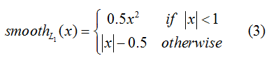
程序中先计算pred和target的差box_diff，而后得到正样本的差in_box_diff（通过乘以权重bbox_inside_weights将负样本设置为0）及绝对值abs_in_box_diff，之后计算上式(3)中的符号smoothL1_sign，并得到的smooth L1 loss：in_loss_box，乘以bbox_outside_weights权重，并得到最终的loss：loss_box。

其中_smooth_l1_loss定义如下：

def _smooth_l1_loss(self, bbox_pred, bbox_targets, bbox_inside_weights, bbox_outside_weights, sigma=1.0, dim=[1]):
    sigma_2 = sigma ** 2
    box_diff = bbox_pred - bbox_targets   # 预测的和真实的相减
    in_box_diff = bbox_inside_weights * box_diff  # 乘以正样本的权重1（rpn：去除负样本和不关注的样本，rcnn：去除负样本）
    abs_in_box_diff = tf.abs(in_box_diff)  # 绝对值
    smoothL1_sign = tf.stop_gradient(tf.to_float(tf.less(abs_in_box_diff, 1. / sigma_2)))   # 小于阈值的截断的标志位
    in_loss_box = tf.pow(in_box_diff, 2) * (sigma_2 / 2.) * smoothL1_sign + (abs_in_box_diff - (0.5 / sigma_2)) * (1. - smoothL1_sign)   # smooth l1 loss
    out_loss_box = bbox_outside_weights * in_loss_box   # rpn：除以有效样本总数（不考虑不关注的样本），进行归一化；rcnn：正样本四个坐标权重为1，负样本为0
    loss_box = tf.reduce_mean(tf.reduce_sum(out_loss_box, axis=dim))
    return loss_box

补充说明

基础网络部分细节

1. 代码中主要使用了两种尺寸，一个是原始图片尺寸，一个是压缩之后的图片尺寸；原始图片进入基础网络之前会被压缩到MxN，但MxN 并不是固定的尺寸，而是把原始图片等比例resize之后的尺寸，源代码里面设置的是压缩到最小边长为600，但是如果压缩之后最大边长超过2000，则以最大边长2000为限制条件。

2. 基础网络部分的说明，其中pooling层kernel_size=2，stride=2。这样每个经过pooling层的MxN矩阵，都会变为(M/2)*(N/2)大小，那么，一个MxN大小的矩阵经过Convlayers中的4次pooling之后尺寸变为(M/16)x(N/16)。那么假设原图为720*1280，MxN为600*1067，基础网络最终的conv5_3 输出为1*38*67*1024。

   也就是说特征图对于原始图像的感受野是16，fead_stride=16

3. 在代码中经常用到的im_info是什么?

   blobs['im_info'] = np.array([im_blob.shape[1], im_blob.shape[2],im_scales[0]]
   

   可以看到，它里面包含了三个元素，图片的width,height，以及im_scales，也就是图片被压缩到600最小边长尺寸时候被压缩的比例，比如以3中提到的为例，它就是0.833

4. Blobs 是什么？ 它里面包含了groundtruth 框数据，图片数据，图片标签的一个字典类型数据，需要说明的是它里面每次只有一张图片的数据，Faster RCNN 整个网络每次只处理一张图片，这是和我们以前接触的网络按照batch处理图片的方式有所区别的；同时，代码中涉及到的 batch_size 不是图片的数量，而是每张图片里面提取出来的框的个数；mini_batch 是从一张图上提取出来的256个anchor，不同的是，caffe 版本的代码是使用2张图片，每张图片128个anchor进行训练。

5. imdb是一个类，它对所有图片名称，路径，类别等相关信息做了一个汇总;

   roidb是imdb的一个属性，里面是一个字典，包含了它的GTbox，以及真实标签和翻转标签。

6. anchor 是什么？

   上面我们已经得到了基础网络最终的conv5_3 输出为1*38*67*1024（1024是层数），在这个特征参数的基础上，通过一个3x3的滑动窗口，在这个38*67的区域上进行滑动，stride=1，padding=2，这样一来，滑动得到的就是38*67个3x3的窗口。

   对于每个3x3的窗口，计算这个滑动窗口的中心点所对应的原始图片的中心点。然后作者假定，这个3x3窗口，是从原始图片上通过SPP池化得到的，而这个池化的区域的面积以及比例，就是一个个的anchor。换句话说，对于每个3x3窗口，作者假定它来自9种不同原始区域的池化，但是这些池化在原始图片中的中心点，都完全一样。这个中心点，就是刚才提到的，3x3窗口中心点所对应的原始图片中的中心点。如此一来，在每个窗口位置，我们都可以根据9个不同长宽比例、不同面积的anchor，逆向推导出它所对应的原始图片中的一个区域，这个区域的尺寸以及坐标，都是已知的。而这个区域，就是我们想要的 proposal。所以我们通过滑动窗口和anchor，成功得到了 38*67x9 个原始图片的proposal。接下来，每个proposal我们只输出6个参数：每个 proposal 和 ground truth 进行比较得到的前景概率和背景概率(2个参数）（对应 cls_score）；由于每个 proposal 和 ground truth 位置及尺寸上的差异，从 proposal 通过平移放缩得到 ground truth 需要的4个平移放缩参数（对应 bbox_pred）。

   最后明确的一点就是在代码中，anchor，proposal，rois ，boxes 代表的含义其实都是一样的，都是推荐的区域或者框，不过有所区别的地方在于这几个名词有一个递进的关系，最开始的是锚定的框 anchor，数量最多有约20000个(根据resize后的图片大小不同而有数量有所变化)，然后是RPN网络推荐的框 proposal，数量较多，train时候有2000个，最后是实际分类时候用到的 rois 框，每张图片有256个；最后得到的结果就是 boxes。

_region_proposal 部分（RPN）

[外链图片转存失败(img-GNx0r4Xo-1566548279862)(C:\F\notebook\faster-rcnn\8.jpg)]

_region_proposal 的下面有三个主要的方法:

• _proposal_layer

​ 主要生成推荐区域proposal和前景背景得分rpn_scores,相当于①上图 部分.

_proposal_layer 有二个主要功能。

​ (1)使用经过rpn网络层后生成的rpn_box_prob把anchor位置进行第一次修正;

​ (2)按照得分排序，取前12000个anchor，再nms,取前面2000个(但是这个数字在test的时候就变成了6000和300，这就是最后结果300个框的来源)。最终返回
proposals , scores，也就是rois, roi_scores。

• _anchor_target_layer

  主要生成第一次anchor的label,rpn_bbox_targets,以及前景背景的label，rpn_labels,相当于上图 ②部分.

  通过对所有的anchor与所有的GT计算IOU，由此得到 rpn_labels(特征图每个位置对应的正样本、负样本还是不关注), rpn_bbox_targets(anchors和anchors对应的正样本计算的坐标偏移), rpn_bbox_inside_weights(前景控制权重), rpn_bbox_outside_weights(背景控制权重，在损失函数中使用)这4个比较重要的第一次目标label，通过消除在图像外部的 anchor，计算IOU >=0.7 为正样本，IOU <0.3为负样本，得到在理想情况下应该各自一半的256个正负样本（实际上正样本大多只有10-100个之间，相对负样本偏少）。

• _proposal_target_layer

  _proposal_target_layer主要功能是计算获得属于最后的分类网络的label。

  生成256个rois的label,以及这些rois的label,bbox_targets,相当于上图③部分.

  使用上一步得到的 proposals , scores，生成最后一步需要的labels, bbox_targets, bbox_inside_weights, bbox_outside_weights。

  因为之前的anchor位置已经修正过了，所以这里又计算了一次经过 proposal_layer 修正后的的box与 GT的IOU来得到label， 但是阈值不一样了，变成了大于等于0.5为1，小于为0，并且这里得到的正样本很少，通常只有2-20个，甚至有0个，并且正样本最多为64个，负样本则有比较多个；相应的也重新计算了一次bbox_targets。

  另外，这个函数的另外一个重要功能就是从RPN网络出来的2000余个rois中挑选256个

_crop_pool_layer 部分（替换Roi Pooling）

这一部分，作者使用了ROIpooling的另外一种实现形式，核心代码如下：

x1 = tf.slice(rois, [0,1], [-1, 1], name="x1") / width
y1 = tf.slice(rois, [0,2], [-1, 1], name="y1") / height
x2 = tf.slice(rois, [0,3], [-1, 1], name="x2") / width
y2 = tf.slice(rois, [0,4], [-1, 1], name="y2") / height
# Won't be back-propagated to rois anyway, but to save time
bboxes = tf.stop_gradient(tf.concat([y1, x1, y2, x2], axis=1))
pre_pool_size = cfg.POOLING_SIZE * 2 #7*2
crops = tf.image.crop_and_resize(bottom,bboxes, tf.to_int32(batch_ids), [pre_pool_size, pre_pool_size],name="crops")
return slim.max_pool2d(crops, [2, 2],padding='SAME')

进入的是：conv5_3 输出为1*38*67*1024， 以及256个rois代表的位置。

输出的是：

Tensor("resnet_v1_101_3/pool5/crops:0",shape=(256, 7, 7, 1024), dtype=float32)

这里可以看到先对rois进行了一个转换操作，h,w是resize后的图像大小，把rois除以h,w就得到了rois在特征图上的位置，然后把conv5_3先crop,就是把roi对应的特征crop出来，然后resize到14*14的大小，resize是为了后面的统一大小，这个操作很有创意，也比较有意思，直接使用了tensorflow的图像处理方法 crop_and_resize 来进行类似 ROI 的操作，最后再做了一个减半的pooling操作，得到7*7的特征图。

其他细节理解

1. 什么是NMS？

   NMS是用来去掉冗余的框的。

   NMS的原理是抑制和当前分数最大的框IOU较高的框。如果阈值设置为0.3， 那么就是所有与当前分数最大的框box的iou小于阈值的得到保留，而大于阈值的box被这个框吸收，也就是被剔除，而只保留当前分数最大的框，然后在下一次重复这个过程，通过去掉当前最大分数的box的可以吸收的box，来一步一步缩减box规模，所以阈值越小，吸收掉的框越多，阈值越大，保留的框越多

2. batch_size 的区别？

   有两个batch size,一个是__C.TRAIN.RPN_BATCHSIZE = 256，这是用在RPN网络里面的，

   num_fg = int(cfg.TRAIN.RPN_FG_FRACTION * cfg.TRAIN.RPN_BATCHSIZE)
   

   另外一个是：

   # Minibatch size (number of regions of interest [ROIs])
   __C.TRAIN.BATCH_SIZE = 256 
   rois_per_image = cfg.TRAIN.BATCH_SIZE / num_images
   

   这个是用在最后的分类网络的，二者的数量都是256，但是后者的正样本比例更少，最多使用 1/4 的 正样本，即64个。

   # Fraction of minibatch that is labeled foreground (i.e. class > 0)
   __C.TRAIN.FG_FRACTION = 0.25
   

3. RPN的样本选取规则和最终Roi Pooling样本选取规则有何不同？

   RPN网络样本选取规则：

   • 对每个标定的真值候选区域，与其重叠比例最大的anchor记为前景样本
   • 对a)剩余的anchor，如果其与某个标定重叠比例大于0.7，记为前景样本；如果其与任意一个标定的重叠比例都小于0.3，记为背景样本；正负样本共256个，最多各占一半
   • 对a),b)剩余的anchor，弃去不用
   • 跨越图像边界的anchor弃去不用

   Roi Pooling样本选取规则：

   • 从 RPN 生成的rois中抽取256个样本
   • 阈值变成了> 0.5 为正， 在 ( 0, 0.5] 区间为负
   • 正样本最多为64个

4. anchor的box_target计算和proposal的box_target的计算的过程有一个细小的差异：

   if cfg.TRAIN.BBOX_NORMALIZE_TARGETS_PRECOMPUTED:
   # Optionally normalize targets by a precomputed mean and stdev
       targets = ((targets - np.array(cfg.TRAIN.BBOX_NORMALIZE_MEANS)) / np.array(cfg.TRAIN.BBOX_NORMALIZE_STDS))
   

   proposal的box_target多一个标准化的过程，BBOX_NORMALIZE_MEANS是全0，没有影响，除以BBOX_NORMALIZE_STDS（0.1,0.1,0.2,0.2）相当于把box_target扩大了10倍和5倍。

   同时有：

   if testing:
       stds = np.tile(np.array(cfg.TRAIN.BBOX_NORMALIZE_STDS), (self._num_classes))
       means = np.tile(np.array(cfg.TRAIN.BBOX_NORMALIZE_MEANS), (self._num_classes))
       self._predictions["bbox_pred"] *= stds
       self._predictions["bbox_pred"] += means
   

   同样的，在测试的时候把这个扩大了10倍的预测框的值修正过来了。

5. bbox_inside_weights, bbox_outside_weights 这两个权重具体是什么意思？

    # Deprecated (outside weights)   
     __C.TRAIN.RPN_BBOX_INSIDE_WEIGHTS = (1.0, 1.0, 1.0, 1.0)
     # only the positive ones have regression targets
     bbox_inside_weights[labels == 1, :] = np.array(cfg.TRAIN.RPN_BBOX_INSIDE_WEIGHTS)
   

   所以可以看出，bbox_inside_weights 它实际上就是控制回归的对象的，只有真正是前景的对象才会被回归。

   # Give the positive RPN examples weight of p * 1 / {num positives}
    # and give negatives a weight of (1 - p)
    # Set to -1.0 to use uniform example weighting
    __C.TRAIN.RPN_POSITIVE_WEIGHT = -1.0  
   
    if cfg.TRAIN.RPN_POSITIVE_WEIGHT < 0:
       # uniform weighting of examples (given non-uniform sampling)
       num_examples = np.sum(labels >= 0)
       positive_weights = np.ones((1, 4)) * 1.0 / num_examples
       negative_weights = np.ones((1, 4)) * 1.0 / num_examples
     else:
       assert ((cfg.TRAIN.RPN_POSITIVE_WEIGHT > 0) &
               (cfg.TRAIN.RPN_POSITIVE_WEIGHT < 1))
       positive_weights = (cfg.TRAIN.RPN_POSITIVE_WEIGHT /
                           np.sum(labels == 1))
       negative_weights = ((1.0 - cfg.TRAIN.RPN_POSITIVE_WEIGHT) /
                           np.sum(labels == 0))
     bbox_outside_weights[labels == 1, :] = positive_weights
     bbox_outside_weights[labels == 0, :] = negative_weights
   

   可以看出，bbox_outside_weights 也是用1/N1, 2/N0 初始化,对前景和背景控制权重，比起上面多了一个背景的权重，从第二步来看， positive_weights ，negative_weights有互补的意味。

   这两个参数都是在 _smooth_l1_loss 里面使用，

   rpn_loss_box = self._smooth_l1_loss(rpn_bbox_pred, rpn_bbox_targets, rpn_bbox_inside_weights,
                                             rpn_bbox_outside_weights, sigma=sigma_rpn, dim=[1, 2, 3])
   box_diff = bbox_pred - bbox_targets
   in_box_diff = bbox_inside_weights * box_diff   
   abs_in_box_diff = tf.abs(in_box_diff)
   smoothL1_sign = tf.stop_gradient(tf.to_float(tf.less(abs_in_box_diff, 1. / sigma_2)))
   in_loss_box = tf.pow(in_box_diff, 2) * (sigma_2 / 2.) * smoothL1_sign \
                     + (abs_in_box_diff - (0.5 / sigma_2)) * (1. - smoothL1_sign)
   out_loss_box = bbox_outside_weights * in_loss_box  ；
   

   可以看出，bbox_outside_weights 就是为了平衡 box_loss,cls_loss 的，因为二个loss差距过大，所以它被设置为 1/N 的权重。

   论文提到的 _smooth_l1_loss 相当于一个二次方函数和直线函数的结合，但是为什么要这样呢？不太懂，论文说它比较鲁棒，没有rcnn中使用的L2 loss 那么对异常值敏感，当回归目标不受控制时候，使用L2 loss 会需要更加细心的调整学习率以避免梯度爆炸？_smooth_l1_loss消除了这个敏感性。

参考网址：

• https://zhuanlan.zhihu.com/p/32230004
• https://www.cnblogs.com/darkknightzh/p/10043864.html#_label2
• https://blog.csdn.net/zzyincsdn/article/details/83989606
• https://www.cnblogs.com/dudumiaomiao/p/6560841.html