【图像处理】MATLAB：频域处理

二维离散傅里叶变换

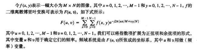
代码示例

f = imread('image.tif');

F = fft2(f);                                                %傅里叶变换,逆变换为 f=ifft2(F),取实部为 f=real(ifft2(F))

S = abs(F);                                                 %傅里叶频谱

Fc = fftshift(F);                                           %将变换的原点移动到频率矩阵的中心,反变换为 F=ifftshift(Fc),
                                                            %频率矩阵中心点位于[floor(M/2)+1,floor(N/2)+1]
S2 = log(1+abs(Fc));                                        %对数变换

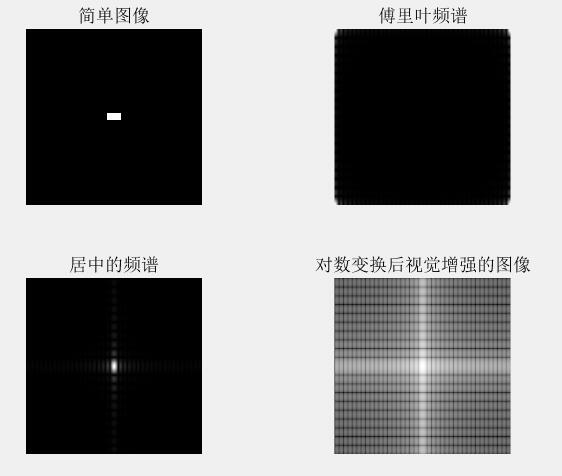
subplot(2,2,1);imshow(f);title('简单图像');
subplot(2,2,2);imshow(S,[ ]);title('傅里叶频谱');
subplot(2,2,3);imshow(abs(Fc),[ ]);title('居中的频谱');
subplot(2,2,4);imshow(S2,[ ]);title('对数变换后视觉增强的图像');

运行结果

---

频域滤波

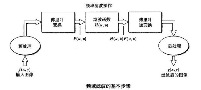
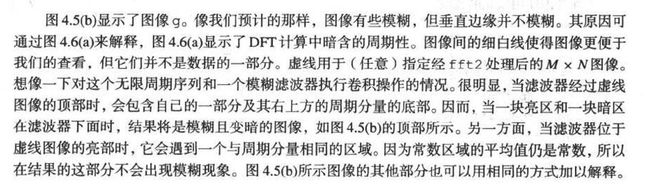
  若使用DFT进行滤波操作，则图像及其变换都将自动地看成是周期性的。若周期关于函数的非零部分的持续时间很靠近，则对周期函数执行卷积运算会导致相邻周期之间的干扰，称之为折叠误差的干扰。可通过使用零来填充函数的方法避免。

  若处理的函数大小均是M×N，则填充值可设置为：P≥2M-1 和 Q ≥2N-1。

  paddedsize函数用于计算满足PQ的最小偶数值，同样也提供一个选项来填充输入图像，以便形成的方形图像的大小等于最接近的2的整数次幂。根据所得出的PQ，可使用函数fft2来计算经零填充后的FFT：

    F = fft2 ( f , PQ ( 1 ) , PQ ( 2 ) )

function PQ = paddedsize(AB, CD, PARAM)
%PADDEDSIZE Computes padded sizes useful for FFT-based filtering. 
%   PQ = PADDEDSIZE(AB), where AB is a two-element size vector,
%   computes the two-element size vector PQ = 2*AB.
%
%   PQ = PADDEDSIZE(AB, 'PWR2') computes the vector PQ such that
%   PQ(1) = PQ(2) = 2^nextpow2(2*m), where m is MAX(AB).
%
%   PQ = PADDEDSIZE(AB, CD), where AB and CD are two-element size
%   vectors, computes the two-element size vector PQ.  The elements
%   of PQ are the smallest even integers greater than or equal to 
%   AB + CD - 1.
%
%   PQ = PADDEDSIZE(AB, CD, 'PWR2') computes the vector PQ such that
%   PQ(1) = PQ(2) = 2^nextpow2(2*m), where m is MAX([AB CD]). 

%   Copyright 2002-2004 R. C. Gonzalez, R. E. Woods, & S. L. Eddins
%   Digital Image Processing Using MATLAB, Prentice-Hall, 2004
%   $Revision: 1.5 $  $Date: 2003/08/25 14:28:22 $

if nargin == 1
   PQ  = 2*AB;
elseif nargin == 2 & ~ischar(CD)
   PQ = AB + CD - 1;
   PQ = 2 * ceil(PQ / 2);
elseif nargin == 2
   m = max(AB); % Maximum dimension.

   % Find power-of-2 at least twice m.
   P = 2^nextpow2(2*m);
   PQ = [P, P];
elseif nargin == 3
   m = max([AB CD]); % Maximum dimension.
   P = 2^nextpow2(2*m);
   PQ = [P, P];
else 
   error('Wrong number of inputs.')
end

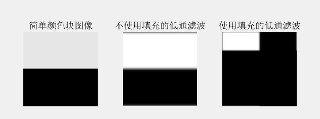
代码示例

f = imread('square.tif');

%不使用填充的频率低通滤波处理
[M,N] = size(f);
F = fft2(f);
sig = 10;
H = lpfilter('gaussian',M,N,sig);   %用于生成高斯低通滤波器
G = H.*F;
g = real(ifft2(G));

%使用填充的频率低通滤波处理
PQ = paddedsize(size(f));                   %获取填充参数
Fp = fft2(f,PQ(1),PQ(2));                   %得到使用填充的傅里叶变换
Hp = lpfilter('gaussian',PQ(1),PQ(2),2*sig);    %高斯低通滤波器
Gp = Hp.*Fp;                                %将变换乘以滤波函数
gp = real(ifft2(Gp));                       %获得傅里叶逆变换的实部
gpc = gp(1:size(f,1),1:size(f,2));          %将左上部的矩形修剪为原始大小

subplot(1,3,1);imshow(f);title('简单颜色块图像');
subplot(1,3,2);imshow(g,[ ]);title('不使用填充的低通滤波');
subplot(1,3,3);imshow(gp,[ ]);title('使用填充的低通滤波');

运行结果

不使用填充对应图像顶边有黑线的解释：

---

空间滤波和频域滤波的比较

  使用空间域滤波和频域滤波得到的图像对所有实用目的来说，都是相同的。

  通常来说，当滤波器较小时，空间滤波要比频域滤波更有效，但是这个“小”的定义比较复杂，取决于众多因素，如所使用算法、缓冲器大小、数据复杂度等。

  函数 freqz2 用于计算FIR滤波器的频率响应。

    H = freqz2 ( h , R , C )

  其中，h是一个二维空间滤波器，H是响应的二维频域滤波器，R为H的行数，C为H的列数。

代码示例

f = imread('bld.tif');
F = fft2(f);
S = fftshift(log(1+abs(F)));
S = gscale(S);

h = fspecial('sobel');
PQ = paddedsize(size(F));
H = freqz2(h,PQ(1),PQ(2));
H1 = ifftshift(H);

gs = imfilter(double(f),h);
gf = dftfilt(f,H1);

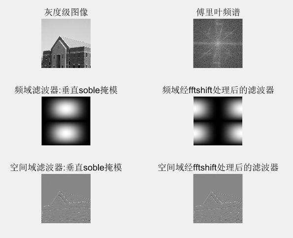
subplot(3,2,1);imshow(f);title('灰度级图像');
subplot(3,2,2);imshow(S);title('傅里叶频谱');
subplot(3,2,3);imshow(abs(H),[ ]);title('频域滤波器:垂直soble掩模');
subplot(3,2,4);imshow(abs(H1),[ ]);title('频域经fftshift处理后的滤波器');
subplot(3,2,5);imshow(gs,[ ]);title('空间域滤波器:垂直soble掩模');
subplot(3,2,6);imshow(gf,[ ]);title('空间域经fftshift处理后的滤波器');

运行结果

---