统计学习方法（三）1-least_sqaure_method

目录

1、最小二乘法拟合曲线

2、正则化

3、简单交叉验证

4、样条插值

1、最小二乘法拟合曲线

[第一章]

最小二乘法

根据高斯-马尔科夫定理,在线性回归模型( $y=\beta x+\epsilon$ )中，如果误差 $\epsilon$ 满足零均值、等方差、互不相关，则最小二乘法估计的回归系数 $\hat{\beta }$ 满足最佳线性无偏估计，即方差最小。

使用最小二乘法拟和曲线

对于数据$(x_i,y_i)(i=1,2,3...,m)$

拟合出函数 $\hat{y}=\hat{w}x$

有误差，即残差：$e_i=\widehat{y_i}-y_i$

残差平方和( ${\sum }_{i=1}^m(\widehat{y_i}-y_i{)}^2$ )最小时 $\hat{y}$ 和 y 相似度最高，更拟合

存在H(x)为n次的多项式，$H(x)=w_0+w_{1}x+w_2{x}^2+...w_n{x}^n={\sum }_{j=1}^n{w}_j{x}^j$

$w(w_0,w_1,w_2,...,w_n)$为参数

最小二乘法就是要找到一组 $w(w_0,w_1,w_2,...,w_n)$ 使得${\sum }_{i=1}^n(h(x_i)-y_i{)}^2$ (残差平方和) 最小

即，求 $min{\sum }_{i=1}^m(h(x_i)-y_i{)}^2$

---

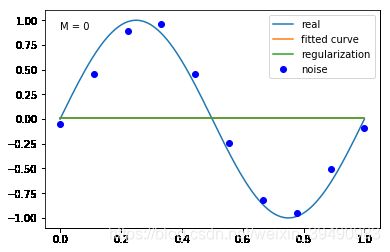
【例1.1 11页】用目标函数$y=sin2\pi x$, 加上一个正太分布的噪音干扰，用多项式去拟合

import numpy as np  #数值计算库
import scipy as sp  #Scipy是一个高级的科学计算库，它和Numpy联系很密切
from scipy.optimize import leastsq  #leastsq()表示最小二乘拟合计算
import matplotlib.pyplot as plt  #画图
%matplotlib inline  
#%matplotlib inline 可以在Ipython编译器里直接使用，功能是可以内嵌绘图，并且可以省略掉plt.show()这一步。

ps: numpy.poly1d([1,2,3]) 生成 $1x^2+2x^1+3x^0$

# 目标函数
def real_func(x):
    return np.sin(2*np.pi*x)  #定义目标函数real_func

# 多项式
def fit_func(p, x):
    f = np.poly1d(p)  #定义多项式，p为参数向量，x为随机变量
    return f(x)

# 残差
def residuals_func(p, x, y):
    ret = fit_func(p, x) - y  #定义残差，即多项式拟合值与实际值的差值，y表示输入变量x对应的实际输出变量
    return ret

# 十个点
x = np.linspace(0, 1, 10)
x_points = np.linspace(0, 1, 1000)
# 加上正态分布噪音的目标函数的值
y_ = real_func(x)
y = [np.random.normal(0, 0.1)+y1 for y1 in y_]

def fitting1(M=0):
    """
    M 为 多项式的最高次数
    """    
    # 随机初始化多项式参数
    p_init = np.random.rand(M+1)
    # 最小二乘法
    p_lsq = leastsq(residuals_func, p_init, args=(x, y))
    
    # 可视化
    plt.plot(x_points, real_func(x_points), label='real')
    plt.plot(x_points, fit_func(p_lsq[0], x_points), label='fitted curve')
    plt.plot(x, y, 'bo', label='noise')
    plt.legend()
    return plt.show()

#M=0
plt.text(0,0.9,"M = 0")  #加入文本注释
fitting1(M=0)

#M=1
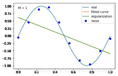
plt.text(0,0.9,"M = 1")
fitting1(M=1)

#M=3
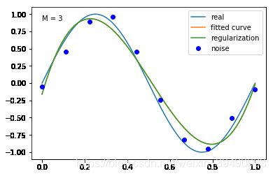
plt.text(0,0.9,"M = 3")
fitting1(M=3)

#M=9
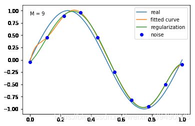
plt.text(0,0.9,"M = 9")
fitting1(M=9)

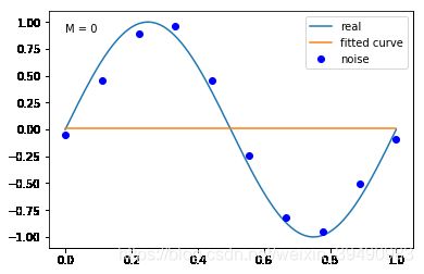
M=0

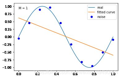
M=1

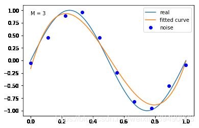
M=3

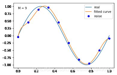
M=9

当M=0时，多项式是一条直线 ，数据的拟合效果很差，认为“欠拟合”，欠拟合通常是因为学习能力低下导致的；

当M=1时，多项式是一条直线 ，数据的拟合效果也很差，认为“欠拟合”；

当M=3时，多项式是一条曲线 ，数据的拟合效果比较好，模型也比较简单；

当M=9时，多项式曲线通过了每个数据点，但模型比较复杂，模型对数据预测过好，对未知数据预测很差，认为“过拟合”，过拟合通常是因为所选择模型的复杂度比真模型更高。

对于欠拟合，只需增加模型复杂度即可；

对于过拟合，常用的方法有：正则化与交叉验证。

2、正则化

结果显示过拟合， 引入正则化项(regularizer)，降低过拟合

$Q(x)={\sum }_{i=1}^n(h(x_i)-y_i{)}^2+\lambda ||w|{|}^2$。

回归问题中，损失函数是平方损失，正则化可以是参数向量的L2范数,也可以是L1范数。

• L1: regularization*abs($p$)

• L2: 0.5 * regularization * np.square($p$)

正则化的作用是选择经验风险与模型复杂度都较小的模型

正则化符合奥卡姆剃刀原理，在所有可能选择的模型中，能够很好的解释已知数据并且十分简单才是最好的模型。

regularization = 0.0001   #作为调整经验风险和正则化项关系的系数

#加入正则化项的结构风险最小化
def residuals_func_regularization(p, x, y):
    ret = fit_func(p, x) - y
    ret = np.append(ret, 0.5*regularization*np.sqrt(np.sum(np.square(p))))  # L2范数作为正则化项
    return ret

# 最小二乘法,加正则化项

def fitting2(M=0):
    """
    M 为 多项式的最高次数
    """    
    # 随机初始化多项式参数
    p_init = np.random.rand(M+1)
    # 最小二乘法
    p_lsq = leastsq(residuals_func, p_init, args=(x, y))
    # 最小二乘法，加入正则化项
    p_lsq_regularization = leastsq(residuals_func_regularization, p_init, args=(x, y))
    
    # 可视化
    plt.plot(x_points, real_func(x_points), label='real')
    plt.plot(x_points, fit_func(p_lsq[0], x_points), label='fitted curve')
    plt.plot(x_points, fit_func(p_lsq_regularization[0], x_points), label='regularization')
    plt.plot(x, y, 'bo', label='noise')
    plt.legend()
    return plt.show()

#M=0
plt.text(0,0.9,"M = 0")  #加入文本注释
fitting2(M=0)

#M=1
plt.text(0,0.9,"M = 1")
fitting2(M=1)

#M=3
plt.text(0,0.9,"M = 3")
fitting2(M=3)

#M=9
plt.text(0,0.9,"M = 9")
fitting2(M=9)

M = 0

M=1

M = 3

M = 9

加入正则化项后，M = 9多项式的拟合效果更好，过拟合降低

3、简单交叉验证

#简单交叉验证，选择有最小预测误差的模型
from sklearn.model_selection import train_test_split


x = np.linspace(0,1,2000)  #创建从0到1，20个等差间隔数列
x_points = np.linspace(0, 1, 1000)  #创建从0到1，个数为1000的等差间隔数列

# 加上正态分布随机噪音的目标函数的值
y_ = real_func(x)  #将创建的等差数列x作为输入，得到目标函数对应的输出值
y = [np.random.normal(0, 0.1)+y1 for y1 in y_]   #解析式，将创建的目标函数的输出值上，随机加入正态分布噪音（其中正态分布的均值为0，标准差为0.1）

test_size = 0.10
seed = 4
x_train,x_test,y_train,y_test = train_test_split(x, y, test_size = test_size, random_state = seed)  #random_stste表示随机种子，为了进行可重复的训练，需要固定random_stste

def fitting3(M=0):
    """
    M 为 多项式的最高次数
    """    
    # 随机初始化多项式参数
    p_init = np.random.rand(M+1)  #来自均匀分布的长度为M+1的随机数，参数表示指定的形状，均匀分布的属于[0, 1)
    # 定义最小二乘法，没有加正则化
    p_lsq = leastsq(residuals_func, p_init, args=(x_train, y_train))  #来自scipy库的leastsq(),表示最小二乘函数，其中residuals_func为指定的误差函数，p_init为参数初始值，args=(x, y)为误差函数中调用的参数
    #leastsq()返回拟合的参数值
    print('Fitting Parameters:', p_lsq[0])  #返回拟合的回归系数
    
    # 可视化
    plt.plot(x_points, real_func(x_points), label='real')
    plt.plot(x_points, fit_func(p_lsq[0], x_points), label='fitted curve')  #拟合的M次多项式
    plt.plot(x_train, y_train, 'bo', label='noise')
    plt.plot(x_test, y_test, 'ro', label='test')
    plt.legend()  #显示图例
    
    
    #训练误差和测试误差
    train_err = np.sum(residuals_func(p_lsq[0],x_train,y_train)**2)/len(x_train)
    test_err = np.sum(residuals_func(p_lsq[0],x_test,y_test)**2)/len(x_test)
    print("训练误差：",train_err)
    print("测试误差：",test_err)
    return p_lsq,train_err,test_err

# M=0，表示多项式次数为0
p_lsq_0 = fitting3(M=0)  #得到的结果为欠拟合

Fitting Parameters: [-0.00254771]
训练误差： 0.5080438309671172
测试误差： 0.5064028740331827

M=0

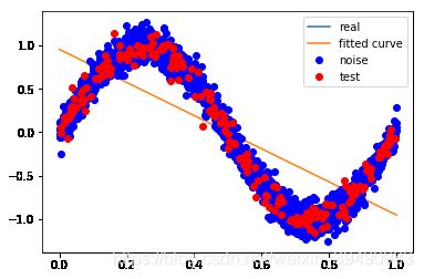
#M = 1
p_lsq_1 = fitting3(M=1)

Fitting Parameters: [-1.9105494 0.95545301]
训练误差： 0.20539699001835074
测试误差： 0.22087267850762224

M=1

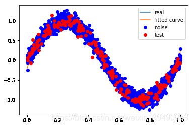
# M=3
p_lsq_3 = fitting3(M=3)

Fitting Parameters: [ 23.18756541 -34.78037548 12.00875189 -0.20806997]
训练误差： 0.014295575398024054
测试误差： 0.015509264503001633

M=3

# M=9
p_lsq_9 = fitting3(M=9)

Fitting Parameters: [-3.30005845e+02 1.55625414e+03 -2.95990953e+03 2.89401400e+03 -1.57115336e+03 5.22004345e+02 -1.20865985e+02 3.11880254e+00 6.58323145e+00 -1.51227081e-02]
训练误差： 0.009914936961862256
测试误差： 0.01022899901075852

M=9

训练误差就是模型在训练集上的误差平均值，度量了模型对训练集拟合的情况。训练误差大说明对训练集特性学习得不够，训练误差太小说明过度学习了训练集特性，容易发生过拟合。

测试误差是模型在测试集上的误差平均值，度量了模型的泛化能力。在实践中，希望测试误差越小越好。

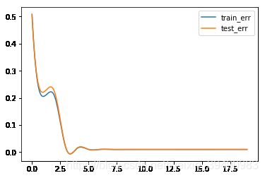
#训练误差，测试误差与模型复杂度，这里我们将多项式次数当作模型复杂度
a = []
b = []
c = []

def err(M=0):
    """
    M 为 多项式的最高次数
    """    
    # 随机初始化多项式参数
    p_init = np.random.rand(M+1)  #来自均匀分布的长度为M+1的随机数，参数表示指定的形状，均匀分布的属于[0, 1)
    # 定义最小二乘法
    p_lsq = leastsq(residuals_func, p_init, args=(x_train, y_train))  #来自scipy库的leastsq(),表示最小二乘函数，其中residuals_func为指定的误差函数，p_init为参数初始值，args=(x, y)为误差函数中调用的参数
    #leastsq()返回拟合的参数值
    
    #训练误差和测试误差
    train_err = np.sum(residuals_func(p_lsq[0],x_train,y_train)**2)/len(x_train)
    test_err = np.sum(residuals_func(p_lsq[0],x_test,y_test)**2)/len(x_test)
    return train_err,test_err

for i in range(0,20):
    train_err = err(M=i)[0]
    test_err = err(M=i)[1]
    a.append(i)
    b.append(train_err)
    c.append(test_err)

from scipy.interpolate import spline
a = np.array(a)
new = np.linspace(a.min(),a.max(),300) #300 represents number of points to make between T.min and T.max
b_smooth = spline(a,np.array(b),new)
c_smooth = spline(a,np.array(c),new)

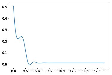
plt.plot(new,b_smooth,label = "train_err")
plt.plot(new,c_smooth,label = "test_err")

plt.legend()  #显示图例

plt.plot(new,b_smooth,label = "train_err")

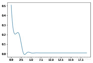
plt.plot(new,c_smooth,label = "test_err")

# M=12
p_lsq_12 = fitting3(M=12)

Fitting Parameters: [ 7.70925250e+02 -2.13948790e+03 1.47955079e+02 5.50179162e+03
-6.90542937e+03 1.62269614e+03 2.85253493e+03 -2.73110094e+03
1.10968608e+03 -2.52646390e+02 1.71394979e+01 5.98163113e+00
-9.12991970e-03]
训练误差： 0.009910459864207754
测试误差： 0.010255984175229287

# M=3
p_lsq_4 = fitting3(M=8)

Fitting Parameters: [ 7.03218670e+01 -1.61073181e+02 3.49309068e+01 1.45531318e+02
-9.15455065e+01 5.06544960e+00 -1.03725482e+01 7.19451627e+00
-2.17477408e-02]
训练误差： 0.009917380173524877
测试误差： 0.010226245482564962

经过简单交叉验证，认为M = 3时，模型效果最好

当模型复杂度增大时，训练误差会减少并趋向于0，测试误差会先减少，达到最小值后又增大。

4、样条插值

插值与拟合的区别：

插值曲线要过数据点，拟合曲线不一定要过数据点。

拟合，就是要得到最接近的结果，是要看总体效果。

import scipy.interpolate
import numpy as np, matplotlib.pyplot as plt
from scipy.interpolate import interp1d

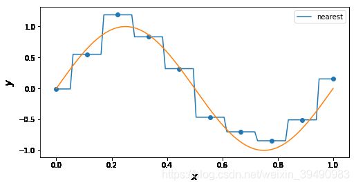
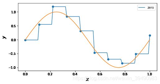
#'nearest','zero'为0阶样条插值 ，'
    #slinear',‘linear’线性插值 相当于1阶样条插值 
    #'quadratic'为2阶样条插值
    #'cubic'3阶样条插值,更高阶的曲线可以直接使用整数值来指定 
    
    
x_ = np.linspace(x.min(), x.max(), 100)
fig, ax = plt.subplots(figsize=(8, 4))
ax.scatter(x, y)
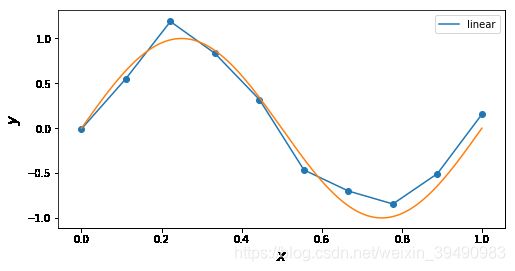
for n in ['linear']:   # 'linear', 'nearest', 'zero', 'slinear', 'quadratic', 'cubic', 5, 9
    f = interp1d(x, y, kind = n)
    ax.plot(x_, f(x_), label= n)
ax.legend()
ax.set_ylabel(r"$y$", fontsize=15)
ax.set_xlabel(r"$x$", fontsize=15)
plt.plot(x_points, real_func(x_points), label='real')
plt.show()

1阶样条/线性插值

x_ = np.linspace(x.min(), x.max(), 100)
fig, ax = plt.subplots(figsize=(8, 4))
ax.scatter(x, y)
for n in [ 'nearest']:   # 'linear', 'nearest', 'zero', 'slinear', 'quadratic', 'cubic', 5, 9
    f = interp1d(x, y, kind = n)
    ax.plot(x_, f(x_), label= n)
ax.legend()
ax.set_ylabel(r"$y$", fontsize=15)
ax.set_xlabel(r"$x$", fontsize=15)
plt.plot(x_points, real_func(x_points), label='real')
plt.show()

0阶样条

x_ = np.linspace(x.min(), x.max(), 100)
fig, ax = plt.subplots(figsize=(8, 4))
ax.scatter(x, y)
for n in [ 'zero']:   # 'linear', 'nearest', 'zero', 'slinear', 'quadratic', 'cubic', 5, 9
    f = interp1d(x, y, kind = n)
    ax.plot(x_, f(x_), label= n)
ax.legend()
ax.set_ylabel(r"$y$", fontsize=15)
ax.set_xlabel(r"$x$", fontsize=15)
plt.plot(x_points, real_func(x_points), label='real')
plt.show()

0阶样条

x_ = np.linspace(x.min(), x.max(), 100)
fig, ax = plt.subplots(figsize=(8, 4))
ax.scatter(x, y)
for n in [ 'slinear']:   # 'linear', 'nearest', 'zero', 'slinear', 'quadratic', 'cubic', 5, 9
    f = interp1d(x, y, kind = n)
    ax.plot(x_, f(x_), label= n)
ax.legend()
ax.set_ylabel(r"$y$", fontsize=15)
ax.set_xlabel(r"$x$", fontsize=15)
plt.plot(x_points, real_func(x_points), label='real')
plt.show()

1阶样条/线性插值

x_ = np.linspace(x.min(), x.max(), 100)
fig, ax = plt.subplots(figsize=(8, 4))
ax.scatter(x, y)
for n in ['quadratic']:   # 'linear', 'nearest', 'zero', 'slinear', 'quadratic', 'cubic', 5, 9
    f = interp1d(x, y, kind = n)
    ax.plot(x_, f(x_), label= n)
ax.legend()
ax.set_ylabel(r"$y$", fontsize=15)
ax.set_xlabel(r"$x$", fontsize=15)
plt.plot(x_points, real_func(x_points), label='real')
plt.show()

2阶样条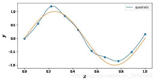

x_ = np.linspace(x.min(), x.max(), 100)
fig, ax = plt.subplots(figsize=(8, 4))
ax.scatter(x, y)
for n in ['cubic']:   # 'linear', 'nearest', 'zero', 'slinear', 'quadratic', 'cubic', 5, 9
    f = interp1d(x, y, kind = n)
    ax.plot(x_, f(x_), label= n)
ax.legend()
ax.set_ylabel(r"$y$", fontsize=15)
ax.set_xlabel(r"$x$", fontsize=15)
plt.plot(x_points, real_func(x_points), label='real')
plt.show()

3阶样条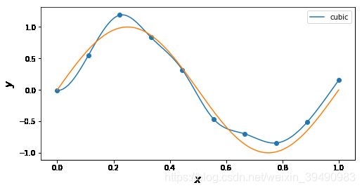

x_ = np.linspace(x.min(), x.max(), 100)
fig, ax = plt.subplots(figsize=(8, 4))
ax.scatter(x, y)
for n in [5]:   # 'linear', 'nearest', 'zero', 'slinear', 'quadratic', 'cubic', 5, 9
    f = interp1d(x, y, kind = n)
    ax.plot(x_, f(x_), label= n)
ax.legend()
ax.set_ylabel(r"$y$", fontsize=15)
ax.set_xlabel(r"$x$", fontsize=15)
plt.plot(x_points, real_func(x_points), label='real')
plt.show()

5阶样条

x_ = np.linspace(x.min(), x.max(), 100)
fig, ax = plt.subplots(figsize=(8, 4))
ax.scatter(x, y)
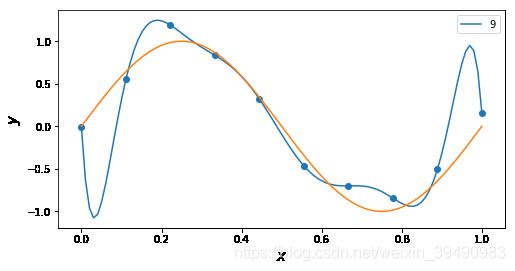
for n in [9]:   # 'linear', 'nearest', 'zero', 'slinear', 'quadratic', 'cubic', 5, 9
    f = interp1d(x, y, kind = n)
    ax.plot(x_, f(x_), label= n)
ax.legend()
ax.set_ylabel(r"$y$", fontsize=15)
ax.set_xlabel(r"$x$", fontsize=15)
plt.plot(x_points, real_func(x_points), label='real')
plt.show()

9阶样条

参考文献：

【1】李航.统计学习方法
【2】github https://github.com/wzyonggege/statistical-learning-method/blob/master/LeastSquaresMethod/least_sqaure_method.ipynb