python混淆矩阵（confusion_matrix）FP、FN、TP、TN、ROC，精确率(Precision),召回率(Recall),准确率(Accuracy)详述与实现

目录

一、FP、FN、TP、TN

二、精确率(Precision),召回率(Recall),准确率(Accuracy)

---

一、FP、FN、TP、TN

你这蠢货，是不是又把酸葡萄和葡萄酸弄“混淆“”啦！！！

上面日常情况中的混淆就是：是否把某两件东西或者多件东西给弄混了，迷糊了。

在机器学习中, 混淆矩阵是一个误差矩阵, 常用来可视化地评估监督学习算法的性能.。混淆矩阵大小为 (n_classes, n_classes) 的方阵, 其中 n_classes 表示类的数量。

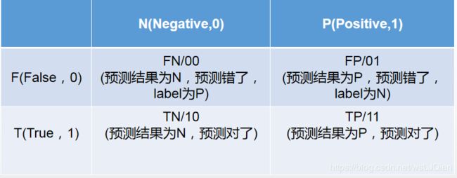
其中，这个矩阵的一行表示预测类中的实例（可以理解为模型预测输出，predict），另一列表示对该预测结果与标签（Ground Truth）进行判定模型的预测结果是否正确，正确为True，反之为False。

在机器学习中ground truth表示有监督学习的训练集的分类准确性，用于证明或者推翻某个假设。有监督的机器学习会对训练数据打标记，试想一下如果训练标记错误，那么将会对测试数据的预测产生影响，因此这里将那些正确打标记的数据成为ground truth。

此时，就引入FP、FN、TP、TN与精确率(Precision)，召回率(Recall)，准确率(Accuracy)。

以猫狗二分类为例，假定cat为正例-Positive，dog为负例-Negative；预测正确为True，反之为False。我们就可以得到下面这样一个表示FP、FN、TP、TN的表：

 此时如下代码所示，其中scikit-learn 混淆矩阵函数 sklearn.metrics.confusion_matrix API 接口，可以用于绘制混淆矩阵

skearn.metrics.confusion_matrix(
    y_true,   # array, Gound true (correct) target values
    y_pred,  # array, Estimated targets as returned by a classifier
    labels=None,  # array, List of labels to index the matrix.
    sample_weight=None  # array-like of shape = [n_samples], Optional sample weights
)

完整示例代码如下：

__author__ = "lingjun"
# E-mail: [email protected]
# welcome to attention:小白CV

import seaborn as sns
from sklearn.metrics import confusion_matrix
import matplotlib.pyplot as plt
sns.set()

f, (ax1,ax2) = plt.subplots(figsize = (10, 8),nrows=2)
y_true = ["dog", "dog", "dog", "cat", "cat", "cat", "cat"]
y_pred = ["cat", "cat", "dog", "cat", "cat", "cat", "cat"]
C2= confusion_matrix(y_true, y_pred, labels=["dog", "cat"])
print(C2)
print(C2.ravel())
sns.heatmap(C2,annot=True)

ax2.set_title('sns_heatmap_confusion_matrix')
ax2.set_xlabel('Pred')
ax2.set_ylabel('True')
f.savefig('sns_heatmap_confusion_matrix.jpg', bbox_inches='tight')

 保存的图像如下所示：

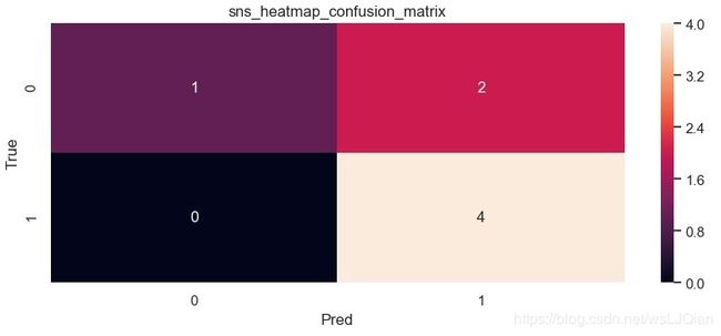
这个时候我们还是不知道skearn.metrics.confusion_matrix做了些什么，这个时候print(C2)，打印看下C2究竟里面包含着什么。最终的打印结果如下所示：

[[1 2]
 [0 4]]
[1 2 0 4]

解释下上面这几个数字的意思：

C2= confusion_matrix(y_true, y_pred, labels=["dog", "cat"])中的labels的顺序就分布是0、1，negative和positive

注：labels=[]可加可不加，不加情况下会自动识别，自己定义

• cat为1-positive，其中真实值中cat有4个，4个被预测为cat，预测正确T，0个被预测为dog，预测错误F；
• dog为0-negative，其中真实值中dog有3个，1个被预测为dog，预测正确T，2个被预测为cat，预测错误F。

所以：TN=1、 FP=2 、FN=0、TP=4。

• TN=1：预测为negative狗中1个被预测正确了
• FP=2 ：预测为positive猫中2个被预测错误了
• FN=0：预测为negative狗中0个被预测错误了
• TP=4：预测为positive猫中4个被预测正确了

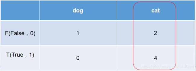
这时候再把上面猫狗预测结果拿来看看，6个被预测为cat，但是只有4个的true是cat，此时就和右侧的红圈对应上了。

y_pred = ["cat", "cat", "dog", "cat", "cat", "cat", "cat"]

y_true = ["dog", "dog", "dog", "cat", "cat", "cat", "cat"]

---

二、精确率(Precision),召回率(Recall),准确率(Accuracy)

有了上面的这些数值，就可以进行如下的计算工作了

准确率(Accuracy):这三个指标里最直观的就是准确率: 模型判断正确的数据(TP+TN)占总数据的比例

"Accuracy: "+str(round((tp+tn)/(tp+fp+fn+tn), 3))

召回率(Recall): 针对数据集中的所有正例label(TP+FN)而言,模型正确判断出的正例(TP)占数据集中所有正例的比例；FN表示被模型误认为是负例但实际是正例的数据；召回率也叫查全率，以物体检测为例,我们往往把图片中的物体作为正例，此时召回率高代表着模型可以找出图片中更多的物体!

"Recall: "+str(round((tp)/(tp+fn), 3))

精确率(Precision):针对模型判断出的所有正例(TP+FP)而言，其中真正例(TP)占的比例。精确率也叫查准率,还是以物体检测为例，精确率高表示模型检测出的物体中大部分确实是物体，只有少量不是物体的对象被当成物体。

"Precision: "+str(round((tp)/(tp+fp), 3))

还有：

("Sensitivity: "+str(round(tp/(tp+fn+0.01), 3)))
("Specificity: "+str(round(1-(fp/(fp+tn+0.01)), 3)))
("False positive rate: "+str(round(fp/(fp+tn+0.01), 3)))
("Positive predictive value: "+str(round(tp/(tp+fp+0.01), 3)))
("Negative predictive value: "+str(round(tn/(fn+tn+0.01), 3)))

三.绘制ROC曲线，及计算以上评价参数

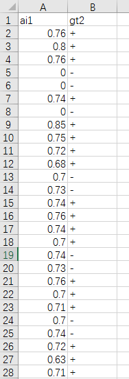
如下为统计数据：

__author__ = "lingjun"
# E-mail: [email protected]
# 微信公众号：小白CV

from sklearn.metrics import roc_auc_score, confusion_matrix, roc_curve, auc
from matplotlib import pyplot as plt
import numpy as np
import torch
import csv

def confusion_matrix_roc(GT, PD, experiment, n_class):
    GT = GT.numpy()
    PD = PD.numpy()

    y_gt = np.argmax(GT, 1)
    y_gt = np.reshape(y_gt, [-1])
    y_pd = np.argmax(PD, 1)
    y_pd = np.reshape(y_pd, [-1])

    # ---- Confusion Matrix and Other Statistic Information ----
    if n_class > 2:
        c_matrix = confusion_matrix(y_gt, y_pd)
        # print("Confussion Matrix:\n", c_matrix)
        list_cfs_mtrx = c_matrix.tolist()
        # print("List", type(list_cfs_mtrx[0]))

        path_confusion = r"./records/" + experiment + "/confusion_matrix.txt"
        # np.savetxt(path_confusion, (c_matrix))
        np.savetxt(path_confusion, np.reshape(list_cfs_mtrx, -1), delimiter=',', fmt='%5s')

    if n_class == 2:
        list_cfs_mtrx = []
        tn, fp, fn, tp = confusion_matrix(y_gt, y_pd).ravel()

        list_cfs_mtrx.append("TN: " + str(tn))
        list_cfs_mtrx.append("FP: " + str(fp))
        list_cfs_mtrx.append("FN: " + str(fn))
        list_cfs_mtrx.append("TP: " + str(tp))
        list_cfs_mtrx.append(" ")
        list_cfs_mtrx.append("Accuracy: " + str(round((tp + tn) / (tp + fp + fn + tn), 3)))
        list_cfs_mtrx.append("Sensitivity: " + str(round(tp / (tp + fn + 0.01), 3)))
        list_cfs_mtrx.append("Specificity: " + str(round(1 - (fp / (fp + tn + 0.01)), 3)))
        list_cfs_mtrx.append("False positive rate: " + str(round(fp / (fp + tn + 0.01), 3)))
        list_cfs_mtrx.append("Positive predictive value: " + str(round(tp / (tp + fp + 0.01), 3)))
        list_cfs_mtrx.append("Negative predictive value: " + str(round(tn / (fn + tn + 0.01), 3)))

        path_confusion = r"./records/" + experiment + "/confusion_matrix.txt"
        np.savetxt(path_confusion, np.reshape(list_cfs_mtrx, -1), delimiter=',', fmt='%5s')

    # ---- ROC ----
    plt.figure(1)
    plt.figure(figsize=(6, 6))

    fpr, tpr, thresholds = roc_curve(GT[:, 1], PD[:, 1])
    roc_auc = auc(fpr, tpr)

    plt.plot(fpr, tpr, lw=1, label="ATB vs NotTB, area=%0.3f)" % (roc_auc))
    # plt.plot(thresholds, tpr, lw=1, label='Thr%d area=%0.2f)' % (1, roc_auc))
    # plt.plot([0, 1], [0, 1], '--', color=(0.6, 0.6, 0.6), label='Luck')

    plt.xlim([0.00, 1.0])
    plt.ylim([0.00, 1.0])
    plt.xlabel("False Positive Rate")
    plt.ylabel("True Positive Rate")
    plt.title("ROC")
    plt.legend(loc="lower right")
    plt.savefig(r"./records/" + experiment + "/ROC.png")
    print("ok")

def inference():
    GT = torch.FloatTensor()
    PD = torch.FloatTensor()
    file = r"Sensitive_rename_inform.csv"
    with open(file, 'r', encoding='UTF-8') as f:
        reader = csv.DictReader(f)
        for row in reader:
            # TODO
            max_patient_score = float(row['ai1'])
            doctor_gt = row['gt2']

            print(max_patient_score,doctor_gt)

            pd = [[max_patient_score, 1-max_patient_score]]
            output_pd = torch.FloatTensor(pd).to(device)

            if doctor_gt == "+":
                target = [[1.0, 0.0]]
            else:
                target = [[0.0, 1.0]]
            target = torch.FloatTensor(target)  # 类型转换, 将list转化为tensor, torch.FloatTensor([1,2])
            Target = torch.autograd.Variable(target).long().to(device)

            GT = torch.cat((GT, Target.float().cpu()), 0)  # 在行上进行堆叠
            PD = torch.cat((PD, output_pd.float().cpu()), 0)

    confusion_matrix_roc(GT, PD, "ROC", 2)

if __name__ == "__main__":
    inference()

若是表格里面有中文，则记得这里进行修改，否则报错

with open(file, 'r') as f:

 

参考资料：

https://baijiahao.baidu.com/s?id=1619821729031070174&wfr=spider&for=pc

https://www.cnblogs.com/klchang/p/9608412.html

https://blog.csdn.net/littlehaes/article/details/83278256

---

小白CV：公众号旨在专注CV（计算机视觉）、AI（人工智能）领域相关技术，文章内容主要围绕C++、Python编程技术，机器学习（ML）、深度学习（DL）、OpenCV等图像处理技术，深度发掘技术要点，记录学习工作中常用的操作，做你学习工作的问题小助手。只关注技术，做CV领域专业的知识分享平台。