需求分析
葡萄牙某银行拟根据现有客户资料建立预测模型,以配合其数据库营销策略,营销方式为电话直销,销售产品为某金融产品(term deposit),数据分析的目标为通过预测模型识别对该金融产品有较高购买意愿的用户群。
数据形式:从数据库中导出的excel文件
数据内容:
# bank client data:
1 - age (numeric)
2 - job : type of job (categorical: "admin.","unknown","unemployed","management","housemaid","entrepreneur","student",
"blue-collar","self-employed","retired","technician","services")
3 - marital : marital status (categorical: "married","divorced","single"; note: "divorced" means divorced or widowed)
4 - education (categorical: "unknown","secondary","primary","tertiary")
5 - default: has credit in default? (binary: "yes","no")
6 - balance: average yearly balance, in euros (numeric)
7 - housing: has housing loan? (binary: "yes","no")
8 - loan: has personal loan? (binary: "yes","no")
# related with the last contact of the current campaign:
9 - contact: contact communication type (categorical: "unknown","telephone","cellular")
10 - day: last contact day of the month (numeric)
11 - month: last contact month of year (categorical: "jan", "feb", "mar", ..., "nov", "dec")
12 - duration: last contact duration, in seconds (numeric)
# other attributes:
13 - campaign: number of contacts performed during this campaign and for this client (numeric, includes last contact)
14 - pdays: number of days that passed by after the client was last contacted from a previous campaign (numeric, -1 means client was not previously contacted)
15 - previous: number of contacts performed before this campaign and for this client (numeric)
16 - poutcome: outcome of the previous marketing campaign (categorical: "unknown","other","failure","success")
Output variable (desired target):
17 - y - has the client subscribed a term deposit? (binary: "yes","no")
下面用R语言进行数据分析及可视化
> bank <- read.csv("H:/bank/bank-full.csv", sep = ";", header = T) //载入数据
> summary(bank) //对数据进行分析汇总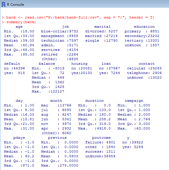
//导入要用到的包
> library(caret)
> library(ggplot2)
> library(gplots)

> require(rpart)
> require(caret)
> require(ggplot2)
> require(gplots)
//运用决策树模型对数据做初步分类建模和变量选择
> bank.tree <- rpart(y ~ ., data = bank, method = "class", cp = 0.001)
> treeImp <- varImp(bank.tree, scale = TRUE, surrogates = FALSE, competes = TRUE)
> treeImp$Variable <- rownames(treeImp)
> treeImp.sort <- treeImp[order(-treeImp$Overall), ]
> ggplot(treeImp, aes(Variable, Overall)) + geom_bar(stat = "identity") + coord_flip()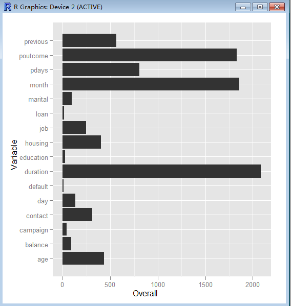
//根据cpplot对树做裁剪
plotcp(bank.tree)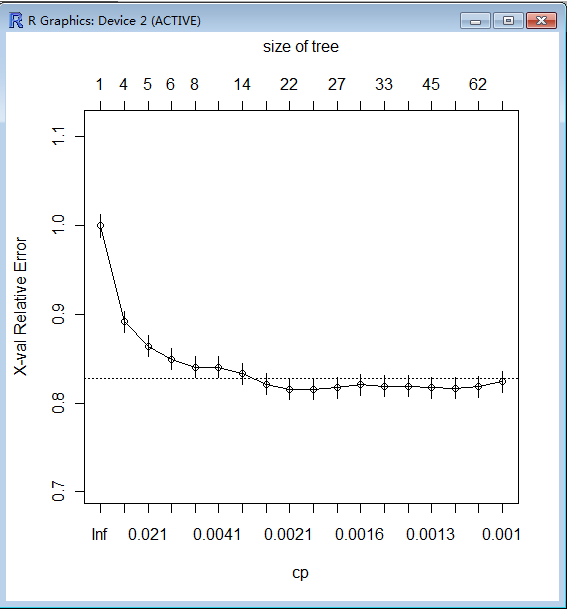
//输出
> printcp(bank.tree)
Classification tree:
rpart(formula = y ~ ., data = bank, method = "class", cp = 0.001)
Variables actually used in tree construction:
[1] age balance contact day duration education housing job marital
[10] month pdays poutcome previous
Root node error: 5289/45211 = 0.11698
n= 45211
CP nsplit rel error xerror xstd
1 0.0380034 0 1.00000 1.00000 0.012921
2 0.0253356 3 0.88599 0.89147 0.012287
3 0.0170164 4 0.86065 0.86425 0.012120
4 0.0080355 5 0.84364 0.84969 0.012028
5 0.0042226 7 0.82757 0.84061 0.011971
6 0.0039705 10 0.81490 0.84061 0.011971
7 0.0034033 13 0.80299 0.83324 0.011924
8 0.0022373 15 0.79618 0.82133 0.011848
9 0.0019537 21 0.78276 0.81584 0.011812
10 0.0017962 24 0.77690 0.81566 0.011811
11 0.0016071 26 0.77330 0.81717 0.011821
12 0.0015126 30 0.76687 0.82057 0.011843
13 0.0014180 32 0.76385 0.81906 0.011833
14 0.0013235 40 0.75099 0.81887 0.011832
15 0.0012290 44 0.74570 0.81755 0.011823
16 0.0011344 51 0.73587 0.81660 0.011817
17 0.0010399 61 0.72452 0.81868 0.011831
18 0.0010000 63 0.72244 0.82416 0.011866
//绘制决策树
> bank.tree <- rpart(y ~ ., data = bank, method = "class", cp = 0.0022373)
> plot(bank.tree, branch = 0, margin = 0.1, uniform = T)
> text(bank.tree, use.n = T, col = "red", cex = 0.6)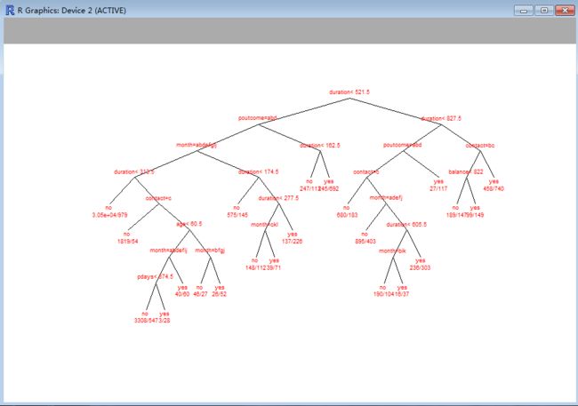
//变量初选,分析和变换
根据决策树分析的结果,我们选择变量重要性最高的前5个变量做进一步研究,依次是:
Duration : last contact duration, in seconds (numeric)
month : last contact month of year (categorical: "jan", "feb", "mar", ..., "nov", "dec")
poutcome : outcome of the previous marketing campaign (categorical: "unknown","other","failure","success")
pdays : number of days that passed by after the client was last contacted from a previous campaign (numeric, -1 means client was not previously contacted)
previous : number of contacts performed before this campaign and for this client (numeric)
//a) Duration参数分析
> bank$y_dummy = ifelse(bank$y == "yes", 1, 0)
> summary(bank$duration)
   Min. 1st Qu.  Median    Mean 3rd Qu.    Max.
    0.0   103.0   180.0   258.2   319.0  4918.0
> ggplot(bank, aes(duration, y_dummy)) + geom_smooth() + geom_point()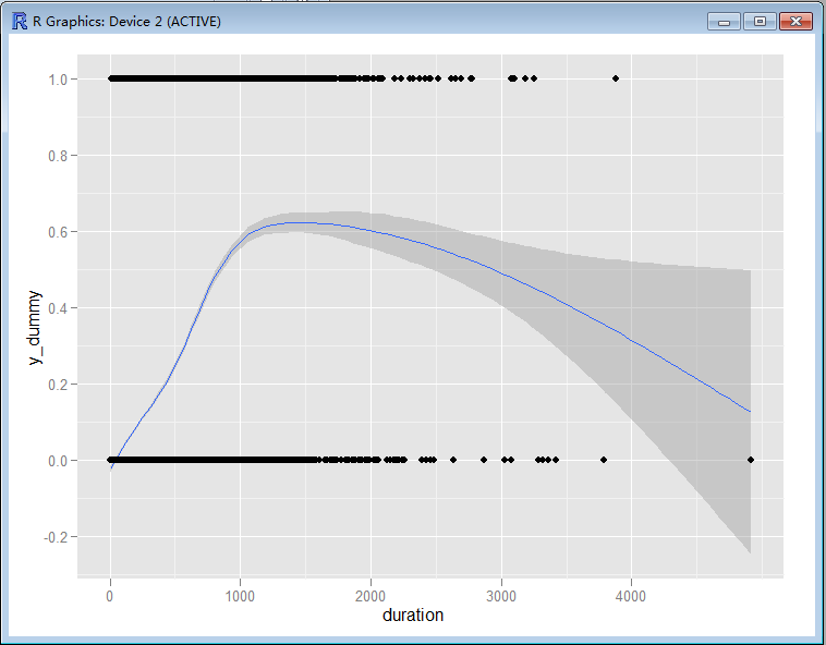
//根据拟合形态对Duration做一个二次项。
> bank$duration.sq <- bank$duration * bank$duration
//b)对month 参数分析
> summary(bank$month)
apr aug dec feb jan jul jun mar may nov oct sep
2932 6247 214 2649 1403 6895 5341 477 13766 3970 738 579
> library(Rcmdr)
> plotMeans(bank$y_dummy, bank$month, error.bars = "se")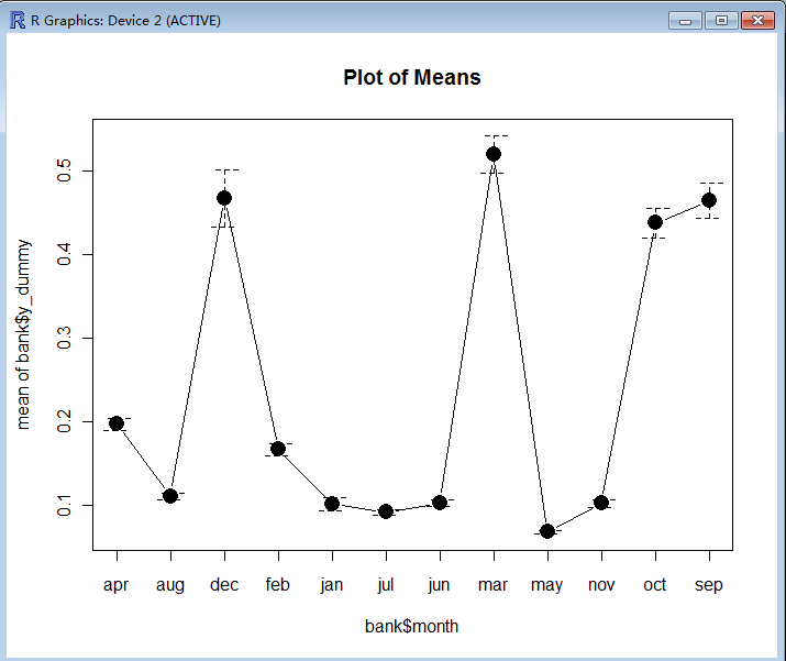
> bank$month.sel <- ifelse(bank$month == "dec", 1, 0)
> bank$month.sel <- ifelse(bank$month == "mar", 1, bank$month)
> bank$month.sel <- ifelse(bank$month == "oct", 1, bank$month)
> bank$month.sel <- ifelse(bank$month == "sep", 1, bank$month)
//c) poutcome参数分析
>summary(bank$poutcome)
failure other success unknown
4901 1840 1511 36959
> plotMeans(bank$y_dummy, bank$poutcome, error.bars = "se")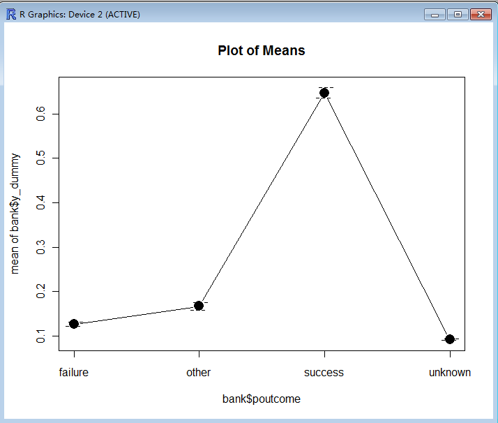
> bank$poutcome.success <- ifelse(bank$poutcome == "success", 1, 0)//d)pdays参数分析
> summary(bank$pdays)
Min. 1st Qu. Median Mean 3rd Qu. Max.
-1.0 -1.0 -1.0 40.2 -1.0 871.0
> bank$nocontact <- ifelse(bank$pdays == -1, 1, 0)
> bank$pdays <- ifelse(bank$pdays == -1, 0, bank$pdays)
> summary(bank$nocontact)
Min. 1st Qu. Median Mean 3rd Qu. Max.
0.0000 1.0000 1.0000 0.8174 1.0000 1.0000
> plotMeans(bank$y_dummy, as.factor(bank$nocontact), error.bars = "se")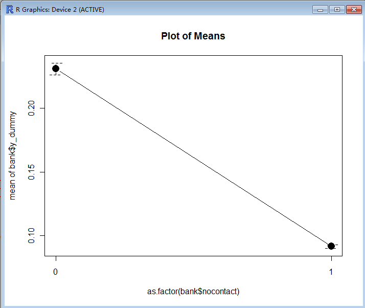
> ggplot(bank, aes(log(pdays + 1))) + geom_histogram()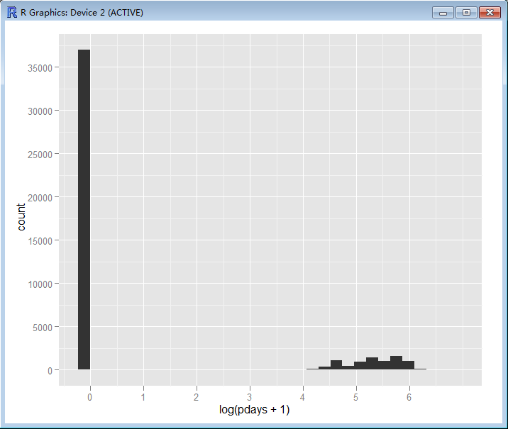
> ggplot(bank, aes(log(pdays + 1), y_dummy)) + geom_smooth() + geom_point()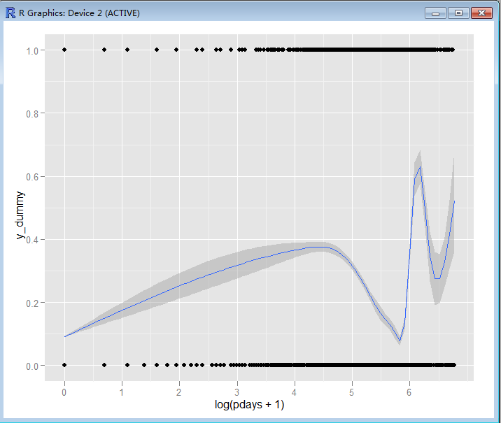
//e) previous参数分析

> summary(bank$previous)
    Min.  1st Qu.   Median     Mean  3rd Qu.     Max.
  0.0000   0.0000   0.0000   0.5803   0.0000 275.0000

> ggplot(bank, aes(log(previous + 1))) + geom_histogram()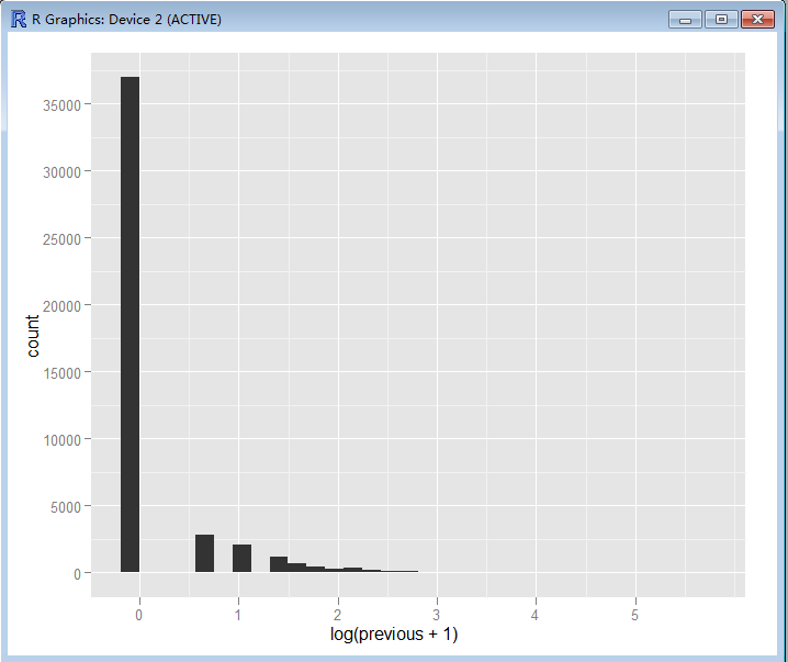
> ggplot(bank, aes(log(previous + 1), y_dummy)) + geom_smooth() + geom_point()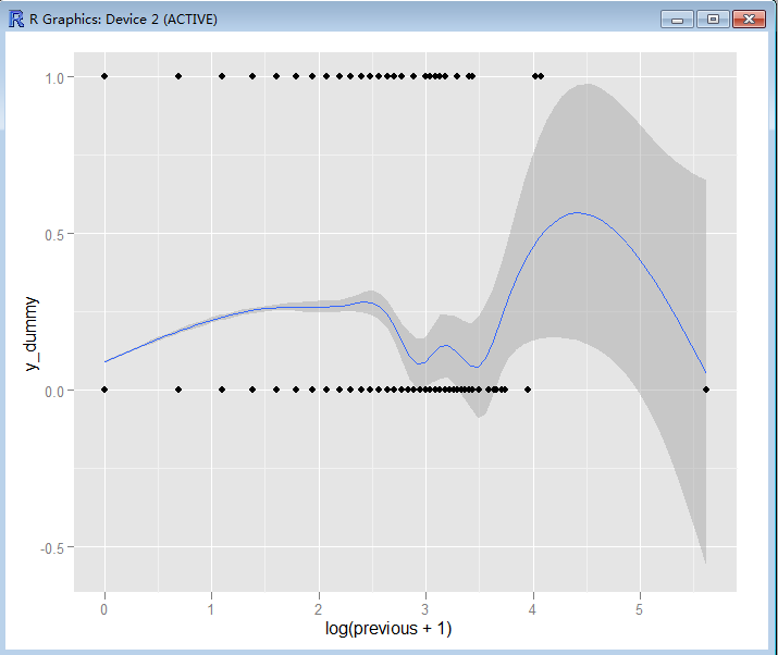
> bank$previous.0 <- as.factor(ifelse(bank$previous == 0, 1, 0))
> bank$previous.1 <- as.factor(ifelse(bank$previous == 1, 1, 0))
> bank$previous.2 <- as.factor(ifelse(bank$previous == 2, 1, 0))
> bank$previous.2plus <- as.factor(ifelse(bank$previous > 2, 1, 0))
//逻辑回归建模
> logistic.full <- glm(y_dummy ~ duration + duration.sq + month.sel + poutcome.success +
+ bank$nocontact + log(pdays + 1) + bank$previous.0 + bank$previous.1 + bank$previous.2 +
+ bank$previous.2plus, data = bank)
> summary(logistic.full)Call:
glm(formula = y_dummy ~ duration + duration.sq + month.sel +
poutcome.success + bank$nocontact + log(pdays + 1) + bank$previous.0 +
bank$previous.1 + bank$previous.2 + bank$previous.2plus,
data = bank)
Deviance Residuals:
Min 1Q Median 3Q Max
-1.15672 -0.11482 -0.04176 0.01313 1.08332
Coefficients: (2 not defined because of singularities)
Estimate Std. Error t value Pr(>|t|)
(Intercept) 1.583e-01 2.348e-02 6.742 1.58e-11 ***
duration 6.574e-04 9.605e-06 68.444 < 2e-16 ***
duration.sq -1.350e-07 6.145e-09 -21.971 < 2e-16 ***
month.sel -6.720e-03 4.346e-04 -15.463 < 2e-16 ***
poutcome.success 4.555e-01 8.085e-03 56.340 < 2e-16 ***
bank$nocontact -1.749e-01 2.336e-02 -7.490 7.04e-14 ***
log(pdays + 1) -2.106e-02 4.335e-03 -4.858 1.19e-06 ***
bank$previous.01 NA NA NA NA
bank$previous.11 -2.522e-02 7.126e-03 -3.540 0.000401 ***
bank$previous.21 -1.641e-02 7.714e-03 -2.128 0.033367 *
bank$previous.2plus1 NA NA NA NA
---
Signif. codes: 0 ‘***’ 0.001 ‘**’ 0.01 ‘*’ 0.05 ‘.’ 0.1 ‘ ’ 1
(Dispersion parameter for gaussian family taken to be 0.07690626)
Null deviance: 4670.3 on 45210 degrees of freedom
Residual deviance: 3476.3 on 45202 degrees of freedom
AIC: 12340
Number of Fisher Scoring iterations: 2
> logistic.step <- step(logistic.full, direction = "both", k = 2)Start: AIC=12340.45
y_dummy ~ duration + duration.sq + month.sel + poutcome.success +
bank$nocontact + log(pdays + 1) + bank$previous.0 + bank$previous.1 +
bank$previous.2 + bank$previous.2plus
Step: AIC=12340.45
y_dummy ~ duration + duration.sq + month.sel + poutcome.success +
bank$nocontact + log(pdays + 1) + bank$previous.0 + bank$previous.1 +
bank$previous.2
Step: AIC=12340.45
y_dummy ~ duration + duration.sq + month.sel + poutcome.success +
bank$nocontact + log(pdays + 1) + bank$previous.1 + bank$previous.2
Df Deviance AIC
- bank$previous.2 1 3476.7 12343
- bank$previous.1 1 3477.3 12351
- log(pdays + 1) 1 3478.1 12362
- bank$nocontact 1 3480.6 12394
- month.sel 1 3494.7 12577
- duration.sq 1 3513.4 12819
- poutcome.success 1 3720.4 15407
- duration 1 3836.6 16797
> summary(logistic.step)Call:
glm(formula = y_dummy ~ duration + duration.sq + month.sel +
poutcome.success + bank$nocontact + log(pdays + 1) + bank$previous.1 +
bank$previous.2, data = bank)
Deviance Residuals:
Min 1Q Median 3Q Max
-1.15672 -0.11482 -0.04176 0.01313 1.08332
Coefficients:
Estimate Std. Error t value Pr(>|t|)
(Intercept) 1.583e-01 2.348e-02 6.742 1.58e-11 ***
duration 6.574e-04 9.605e-06 68.444 < 2e-16 ***
duration.sq -1.350e-07 6.145e-09 -21.971 < 2e-16 ***
month.sel -6.720e-03 4.346e-04 -15.463 < 2e-16 ***
poutcome.success 4.555e-01 8.085e-03 56.340 < 2e-16 ***
bank$nocontact -1.749e-01 2.336e-02 -7.490 7.04e-14 ***
log(pdays + 1) -2.106e-02 4.335e-03 -4.858 1.19e-06 ***
bank$previous.11 -2.522e-02 7.126e-03 -3.540 0.000401 ***
bank$previous.21 -1.641e-02 7.714e-03 -2.128 0.033367 *
---
Signif. codes: 0 ‘***’ 0.001 ‘**’ 0.01 ‘*’ 0.05 ‘.’ 0.1 ‘ ’ 1
(Dispersion parameter for gaussian family taken to be 0.07690626)
Null deviance: 4670.3 on 45210 degrees of freedom
Residual deviance: 3476.3 on 45202 degrees of freedom
AIC: 12340
Number of Fisher Scoring iterations: 2
//模型scoring和ROC评估
> require(ROCR)
载入需要的程辑包:ROCR
> bank.pred<-1/(1+exp(-predict(logistic.step)))
> roc.data <- prediction(bank.pred, labels = bank$y)
> roc.data <- performance(roc.data, "tpr", "fpr")
> plot(roc.data)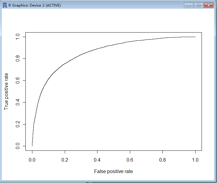
> score<-data.frame("prob.y"=bank.pred,"y"=as.factor(bank$y_dummy))
>ggplot(score, aes(x=prob.y, fill=y)) + geom_histogram(position="identity", binwidth=0.01,alpha=0.5)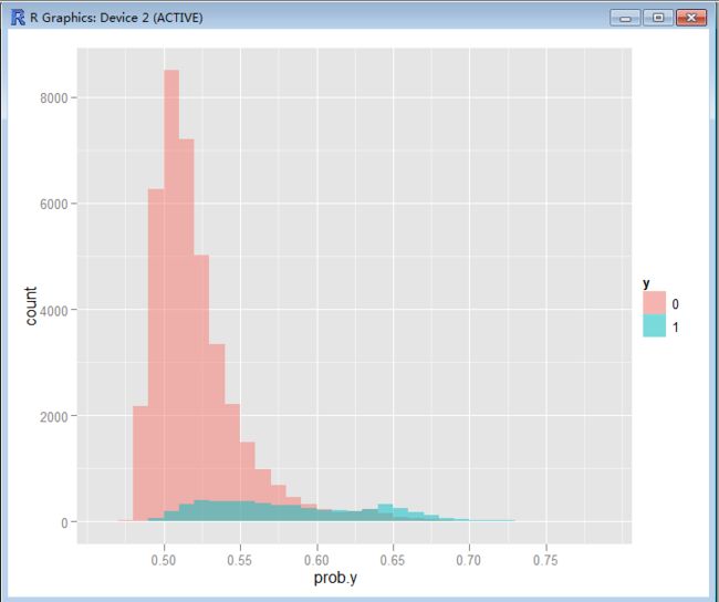
通过对ROC和Score分布的分析,逻辑回归Score的分类效果还是不错的。具体的score cutoff值需要根据业务要求和营销成本而定。