tensorflow2.0实例教程2--keras图像分类

基本分类器：分类衣物图片

这篇教程将会训练一个神经网络模型来对衣物图片进行分类。

如果你了解整个代码的细节也没有什么问题，因为文章的目的在于帮助你快速理清tensorflow构建模型的过程。

这里采用的tf.keras API。

在tensorflow中，keras是一个用来构建和训练模型的高级API接口。

# TensorFlow and tf.keras
import tensorflow as tf
from tensorflow import keras

# Helper libraries
import numpy as np
import matplotlib.pyplot as plt

print(tf.__version__)

2.1.0

导入数据集

fashion_mnist = keras.datasets.fashion_mnist

(train_images, train_labels), (test_images, test_labels) = fashion_mnist.load_data()

load_data()加载数据集返回四个Numpy 数组：

• train_images和train_tags数组是训练集—模型用于训练的数据。
• test_images和test_tags数组是模型测试的测试集。

图像是28x28个NumPy数组，像素值从0到255。标签是一个整数数组，范围从0到9。这些对应于图像所代表的服装类别:

Label	Class
0	T-shirt/top
1	Trouser
2	Pullover
3	Dress
4	Coat
5	Sandal
6	Shirt
7	Sneaker
8	Bag
9	Ankle boot

每个图像被映射到一个标签。由于类名没有包含在数据集中，所以将它们存储在这里，以便以后绘制图像时使用:

class_names = ['T-shirt/top', 'Trouser', 'Pullover', 'Dress', 'Coat',
               'Sandal', 'Shirt', 'Sneaker', 'Bag', 'Ankle boot']

查看一下数据的特征和相关信息

在训练模型之前，让我们先研究一下数据集的格式。如下图所示，训练集中有60000张图像，每张图像表示为28x28像素:

print(train_images.shape)

(60000, 28, 28)

同样的，训练集中有60000个标签:

print(len(train_labels))

60000

每个标签都是0到9之间的整数,分别对应着数据集的10个类别:

print(train_labels)

array([9, 0, 0, ..., 3, 0, 5], dtype=uint8)

测试集中有10,000张图像。同样，每个图像表示为28 x 28像素:

print(test_images.shape)

(10000, 28, 28)

同时，测试集包含10000张图片标签:

print(len(test_labels))

10000

 

预处理数据

在对网络进行训练之前，必须对数据进行预处理。

如果你输出并查看训练集中的第一个图像，你会看到像素值落在0到255的范围内:

plt.figure()
plt.imshow(train_images[0])
plt.colorbar()
plt.grid(False)
plt.show()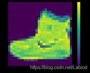

 

在将这些值提供给神经网络模型之前，将这些值缩放到0到1的范围。为此，将这些值除以255。

并且，训练集和测试集以同样的方式进行预处理:

train_images = train_images / 255.0

test_images = test_images / 255.0

为了验证数据的格式是否正确，以用来准备构建和训练网络，我们显示来自训练集的前25个图像，并在每个图像下面显示类名。

plt.figure(figsize=(10,10))
for i in range(25):
    plt.subplot(5,5,i+1)
    plt.xticks([])
    plt.yticks([])
    plt.grid(False)
    plt.imshow(train_images[i], cmap=plt.cm.binary)
    plt.xlabel(class_names[train_labels[i]])
plt.show()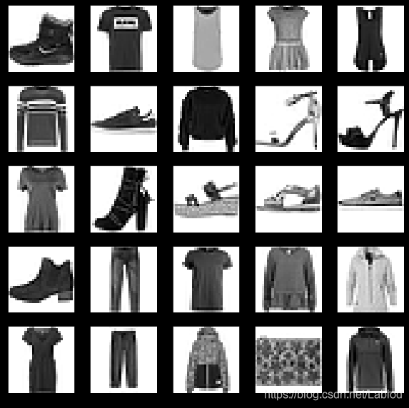

 

构建模型

 构建神经网络需要对模型的层进行选择并搭建，然后对模型进行编译。

设计网络层数

神经网络的基本构件是层（layer）。层(layers)从提供给它们的数据中提取数据的特征表示。希望这些特征表示对我们待解决的问题有一定帮助。

大多数深度学习都是将简单的层次链接在一起。大多数层，比如tf.keras.layers.Dense, 都具有在训练中学习的参数。

model = keras.Sequential([
    keras.layers.Flatten(input_shape=(28, 28)),
    keras.layers.Dense(128, activation='relu'),
    keras.layers.Dense(10)
])

这个网络的第一层，tf.keras.layers.Flatten，作用是将图像的格式从一个二维数组(28×28像素)转换为一个一维数组(28*28=784像素)。可以把这层想象成把图像中的像素行分解并排列成一行。这一层没有需要学习的参数;它只会重新格式化数据。

在图像像素被展平成一维之后，网络由两个tf.keras.layers.Dense组成的序列组成，这些层是紧密相连的，或完全相连的神经层。第一个致密层有128个节点(或神经元)。第二层(也是最后一层)返回长度为10的logits数组。每个节点包含一个（运算后获得的）得分，用来表示当前图像属于10个类中的哪一个。

编译模型

模型准备好进行训练之前，还需要更多的设置来配置训练过程。这些配置方法是在模型的编译步骤中添加的:

• 损失函数——测量模型在训练过程中的准确性。我们希望最小化这个函数，以将模型“引导”到正确的方向。
• 优化器——这是根据模型所看到的数据及其损失函数更新模型的方法。
• 度量标准——用于监视训练和测试步骤。接下来的例子里使用了准确率作为评价指标，准确率的含义就是被正确分类的图像的比例。

model.compile(optimizer='adam',
              loss=tf.keras.losses.SparseCategoricalCrossentropy(from_logits=True),
              metrics=['accuracy'])

 

训练模型

 训练神经网络模型需要以下几个流程:

1. 将训练数据提供给模型。在本例中，训练数据位于train_images和train_tags数组中。
2. 模型学会将图像和标签联系起来。
3. 模型在测试集上预测结果。在这个例子中，测试集是test_images数组。
4. 验证预测是否与test_labels数组中的标签匹配。

给模型提供训练数据

 要开始训练过程的话，我们调用 model.fit 方法——之所以这么叫，是因为它将模型“适合（fit）”于训练数据:

model.fit(train_images, train_labels, epochs=10)

Train on 60000 samples
Epoch 1/10
60000/60000 [==============================] - 4s 61us/sample - loss: 0.4991 - accuracy: 0.8244
Epoch 2/10
60000/60000 [==============================] - 3s 53us/sample - loss: 0.3771 - accuracy: 0.8643
Epoch 3/10
60000/60000 [==============================] - 3s 53us/sample - loss: 0.3381 - accuracy: 0.8775
Epoch 4/10
60000/60000 [==============================] - 3s 53us/sample - loss: 0.3145 - accuracy: 0.8840
Epoch 5/10
60000/60000 [==============================] - 3s 53us/sample - loss: 0.2950 - accuracy: 0.8908
Epoch 6/10
60000/60000 [==============================] - 3s 52us/sample - loss: 0.2805 - accuracy: 0.8956
Epoch 7/10
60000/60000 [==============================] - 3s 53us/sample - loss: 0.2691 - accuracy: 0.9007
Epoch 8/10
60000/60000 [==============================] - 3s 53us/sample - loss: 0.2580 - accuracy: 0.9044
Epoch 9/10
60000/60000 [==============================] - 3s 53us/sample - loss: 0.2490 - accuracy: 0.9071
Epoch 10/10
60000/60000 [==============================] - 3s 53us/sample - loss: 0.2381 - accuracy: 0.9096

 当模型训练时，显示损失和精度指标。该模型对训练数据的准确率约为0.91(或91%)。

验证精度

 接下来，比较模型在测试数据集上的执行情况:

test_loss, test_acc = model.evaluate(test_images,  test_labels, verbose=2)

print('\nTest accuracy:', test_acc)

10000/10000 - 1s - loss: 0.3548 - accuracy: 0.8802

Test accuracy: 0.8802

结果表明，测试数据集上的精度比训练数据集上的精度略低一些。这种训练精度和测试精度之间的差距表示过度拟合。当机器学习模型在新的、以前不可见的输入上的表现不如在训练数据上的表现时，就会发生过度拟合。过度拟合的模型会“记住”训练数据集中的噪声和细节，从而对模型在新数据上的性能产生负面影响。

有关更多信息，请参见后续博客。

看看预测结果怎么样

通过训练模型，您可以使用它对一些图像进行预测。模型的线性输出，对数。附加一个softmax层，将logits转换为更容易解释的概率。

probability_model = tf.keras.Sequential([model, 
                                         tf.keras.layers.Softmax()])

predictions = probability_model.predict(test_images)

 这里，模型已经预测出了测试集中每张图片的标签，让我们看一下测试集中第一个元素预测的结果。

print(predictions[0])

 输出结果：

array([9.6798196e-09, 3.9551045e-12, 1.1966002e-09, 6.4597640e-11,
       6.9501125e-09, 1.3103469e-04, 1.2785731e-07, 2.0190427e-01,
       1.3739854e-09, 7.9796457e-01], dtype=float32)

 其中，一个预测的输出结果是一个由10个数字组成的数组。它们代表了模型在各个维度预测结果的“置信度（信息，或者概率）”，即图像对应于10件不同的衣服中的每一件的概率。

你可以通过输出看到哪个标签的置信度最高:

print(np.argmax(predictions[0]))

9

 因此，模型最确信这个图像是一个ankle boot，即class_names[9]。通过输出测试标签来对比一下，可以看出这种分类是正确的:

print(test_labels[0])

9

 绘制这张图来查看完整的10个类预测。

def plot_image(i, predictions_array, true_label, img):
  predictions_array, true_label, img = predictions_array, true_label[i], img[i]
  plt.grid(False)
  plt.xticks([])
  plt.yticks([])

  plt.imshow(img, cmap=plt.cm.binary)

  predicted_label = np.argmax(predictions_array)
  if predicted_label == true_label:
    color = 'blue'
  else:
    color = 'red'

  plt.xlabel("{} {:2.0f}% ({})".format(class_names[predicted_label],
                                100*np.max(predictions_array),
                                class_names[true_label]),
                                color=color)

def plot_value_array(i, predictions_array, true_label):
  predictions_array, true_label = predictions_array, true_label[i]
  plt.grid(False)
  plt.xticks(range(10))
  plt.yticks([])
  thisplot = plt.bar(range(10), predictions_array, color="#777777")
  plt.ylim([0, 1])
  predicted_label = np.argmax(predictions_array)

  thisplot[predicted_label].set_color('red')
  thisplot[true_label].set_color('blue')

 

验证精度

通过训练模型，您可以使用它对一些图像进行预测。

让我们看看第0张图片、预测和预测数组。正确的预测标签是蓝色的，错误的预测标签是红色的。这个数字给出了预测标签的百分比(100)。

i = 0
plt.figure(figsize=(6,3))
plt.subplot(1,2,1)
plot_image(i, predictions[i], test_labels, test_images)
plt.subplot(1,2,2)
plot_value_array(i, predictions[i],  test_labels)
plt.show()

 

i = 12
plt.figure(figsize=(6,3))
plt.subplot(1,2,1)
plot_image(i, predictions[i], test_labels, test_images)
plt.subplot(1,2,2)
plot_value_array(i, predictions[i],  test_labels)
plt.show()

 

让我们用所得到的预测值绘制几幅图像。但是要注意，即使在预测结果很高的情况下，模型的判断也可能是错误的。

# Plot the first X test images, their predicted labels, and the true labels.
# Color correct predictions in blue and incorrect predictions in red.
num_rows = 5
num_cols = 3
num_images = num_rows*num_cols
plt.figure(figsize=(2*2*num_cols, 2*num_rows))
for i in range(num_images):
  plt.subplot(num_rows, 2*num_cols, 2*i+1)
  plot_image(i, predictions[i], test_labels, test_images)
  plt.subplot(num_rows, 2*num_cols, 2*i+2)
  plot_value_array(i, predictions[i], test_labels)
plt.tight_layout()
plt.show()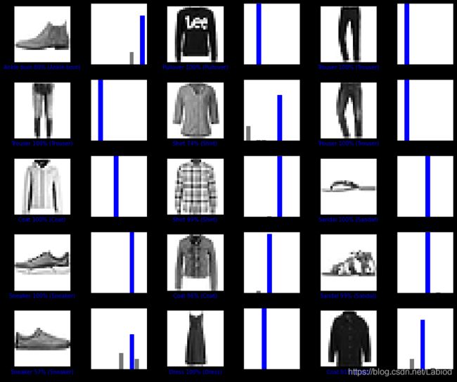

 

使用训练的模型来分类一些其它的图片

最后，利用训练后的模型对单个图像进行预测。

# Grab an image from the test dataset.
img = test_images[1]

print(img.shape)

(28, 28)

Tf.keras模型经过优化，可以(也只能)一次对一批或一组示例进行预测。因此，即使你使用的是一张图片，你也需要把它添加到一个列表中:

# Add the image to a batch where it's the only member.
img = (np.expand_dims(img,0))

print(img.shape)

(1, 28, 28)

 现在预测这张图片的正确标签:

predictions_single = probability_model.predict(img)

print(predictions_single)

 输出：

[[1.1843847e-05 2.8502357e-11 9.9778062e-01 3.2734149e-10 2.0844834e-03
  3.5600198e-15 1.2303848e-04 1.4568713e-08 3.6617865e-11 5.2883337e-14]]

plot_value_array(1, predictions_single[0], test_labels)
_ = plt.xticks(range(10), class_names, rotation=45)

keras.Model.predict 返回—批数据中的每个图像预测结果列表中的一个列表。

输出一个的图片的预测值（取最大可能预测结果为最大值）:

print(np.argmax(predictions_single[0])) # Output one of prediction value arrays

2

可见模型预测了一个我们预期的标签。

关于这里使用的数据集

本文使用了Fashion MNIST的数据集，其中包含10个类别的70,000张灰度图像。

Fashion MNIST是作为经典MNIST数据集的替代产品，通常被用作计算机视觉机器学习程序的“Hello World”。MNIST数据集包含手写数字(0、1、2等)的图像。

本指南使用时尚MNIST来增加多样性，因为它比一般的MNIST更具有挑战性。这两个数据集都相对较小，用于验证算法是否按预期工作。它们是测试和调试代码的良好起点。

这里，使用60,000张图像来训练网络，并使用10,000张图像来评估网络学习如何准确地对图像进行分类。你可以直接从TensorFlow访问Fashion MNIST，从而直接从TensorFlow导入和加载Fashion MNIST数据。