数据分析业务逻辑

本文参考资料有：DataWhale《动手学数据分析》及互联网资源

本章难点突破：

• 数据分块读取
• 文本类数据标签转换
• 正则表达式应用于提取构建新的字符类特征
• 数据表的合并

难点补充学习

1.读取数据

载入数据时我们应当了解数据的存储格式，常见文件后缀有.txt, .xlsx, .csv, .json ，以上格式数据可使用pandas下的read_table,read_csv和read_json读取。如果数据量过大，还可设置具体的按块读取。

2.认识数据

当我们拿到数据表时，首先应当学会认识它们。回想我们使用excl浏览数据时观察的数据维度，可发现行（row），列（column）标签，各列的总数据量、是否存在null值、它们的数据类型，每个数据表的首尾几列数据都是我们认识数据的第一步。在python中，我们使用data.info()查看数据板信息，data.head()和data.tail()查看首尾数据，data.isnull()查看null值数据，data.describe()查看描述性统计分析等。初步了解数据行列信息及数据空值，数据类型情况后我们需要对数据表按条件处理，接下来会涉及数据的删除、填充、筛选、新数据列的形成、新数据关系维度表建立等。

3.数据处理

• 删除

#删除列
del df['a']
df.drop(['PassengerId','Name','Age','Ticket'],axis=1).head(3)

• 填充
• 排序

frame.sort_values(by='c',ascending=False)
frame.sort_index(axis=1,ascendign=False)
frame.sort_values(by=['a','c'])

• 筛选

print((df["Age"]<10).head(3))
midage=df[(df["Age"]>10)&(df["Age"]<50)]
midage=midage.reset_index(drop=True)
print(midage.head(3))
print(midage.loc[[100],['Pclass','Sex']])
print(midage.loc[[100,105,108],['Pclass','Name','Sex']])
print(midage.iloc[[100,105,108],[2,3,4])

• 新列
• 新表

4.构建特征

对特征进行观察，可将其按数据类型（文本型、数值型等）分类，数值型数据可直接用于模型训练，文本型数据则需转换为数值型特征。

• 数值型分箱

df['AgeBand']=pd.cut(df['Age'],5,labels=['1','2','3','4','5'])
df['AgeBand']=pd.cut(df['Age'],[0,5,15,30,50,80],labels=['1','2','3','4','5'])
df['AgeBand']=pd.qcut(df['Age'],[0,0.1,0.3,0.5,0.7,0.9],labels=['1','2','3','4','5'])

• 文本型转换

#将类别文本转换为12345

#方法一: replace
df['Sex_num'] = df['Sex'].replace(['male','female'],[1,2])
df.head()

#方法二: map
df['Sex_num'] = df['Sex'].map({'male': 1, 'female': 2})
df.head()

#方法三: 使用sklearn.preprocessing的LabelEncoder
from sklearn.preprocessing import LabelEncoder
for feat in ['Cabin', 'Ticket']:
    lbl = LabelEncoder()  
    label_dict = dict(zip(df[feat].unique(), range(df[feat].nunique())))
    df[feat + "_labelEncode"] = df[feat].map(label_dict)
    df[feat + "_labelEncode"] = lbl.fit_transform(df[feat].astype(str))

df.head()

#将类别文本转换为one-hot编码

#方法一: OneHotEncoder
for feat in ["Age", "Embarked"]:
#     x = pd.get_dummies(df["Age"] // 6)
#     x = pd.get_dummies(pd.cut(df['Age'],5))
    x = pd.get_dummies(df[feat], prefix=feat)
    df = pd.concat([df, x], axis=1)
    #df[feat] = pd.get_dummies(df[feat], prefix=feat)
    
df.head()

• 从纯文本Name特征里提取出Titles的特征(所谓的Titles就是名字中的Mr,Miss,Mrs等)

df['Title']=df.Name.str.extract('([A-Za-z]+)\.',expand=False)
print(df.head())




   PassengerId  Survived  Pclass  ... Embarked AgeBand  Title
0            1         0       3  ...        S       2     Mr
1            2         1       1  ...        C       5    Mrs
2            3         1       3  ...        S       3   Miss
3            4         1       1  ...        S       4    Mrs
4            5         0       3  ...        S       4     Mr

[5 rows x 14 columns]
[Finished in 1.6s]

• 将两个表按横纵方向合并

#使用concat
text_left_up = pd.read_csv("C:/Users/HP/Desktop/doc/data/u2/data/train-left-up.csv")
text_left_down = pd.read_csv("C:/Users/HP/Desktop/doc/data/u2/data/train-left-down.csv")
text_right_up = pd.read_csv("C:/Users/HP/Desktop/doc/data/u2/data/train-right-up.csv")
text_right_down = pd.read_csv("C:/Users/HP/Desktop/doc/data/u2/data/train-right-down.csv")

list_up=[text_left_down,text_right_down]
result_up=pd.concat(list_up,axis=1)
print(result_up.head())

list_down=[text_left_down,text_right_down]
result_down=pd.concat(list_down,axis=1)
result=pd.concat([result_up,result_down])
print(result.head())

#使用DataFrame的join和append
result_up=text_left_up.join(text_right_up)
result_down=text_left_down.join(text_right_down)
result=result_up.append(result_down)
print(result.head())

#使用DataFrame的merge方法和append
result_up=pd.merge(text_left_up,text_right_up,left_index=True,right_index=True)
result_down=pd.merge(text_left_down,text_right_down,left_index=True,right_index=True)
result=result_up.append(result_down)
print(result.head())

• 计算数值得到新特征

text=pd.read_csv('C:/Users/HP/Desktop/doc/data/u2/result.csv')
df=text['Fare'].groupby(text['Sex'])
means=df.mean()
print(means)

survived_sex=text['Survived'].groupby(text['Sex']).sum()
print(survived_sex.head())

survived_pclass=text['Survived'].groupby(text['Pclass'])
print(survived_pclass.sum())

print(text.groupby(['Pclass','Age'])['Fare'].mean().head())

result=pd.merge(means,survived_sex,on='Sex')
print(result)

survived_age=text['Survived'].groupby(text['Age']).sum()
survived_age[survived_age.values==survived_age.max()]

5.数据可视化

这里将学习【Seaborn和Matplotlib】，Seaborn相比matplotlib封装了一些对数据的组合和识别的功能；用Seaborn出一些针对seaborn的图表是很快的，比如说分布图、热图、分类分布图等。如果用matplotlib需要先group by先分组再出图；

import numpy as np
import pandas as pd
import matplotlib.pyplot as plt 
text=pd.read_csv(r'C:/Users/HP/Desktop/doc/data/u2/result.csv')
print(text.head())
sex=text.groupby('Sex')['Survived'].sum()
sex.plot.bar()#柱状图
plt.title('survived_count')
plt.show() 

 

#比例柱状图
text.groupby(['Sex','Survived'])['Survived'].count().unstack().plot(kind='bar',stacked='True')
plt.title('survived_count')
plt.ylabel('count')

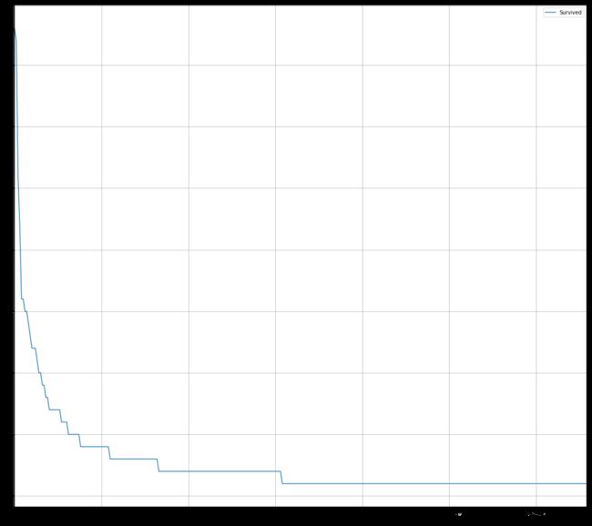
#排序后绘折线图
fare_sur=text.groupby(['Fare'])['Survived'].value_counts().sort_values(ascending=False)

fig=plt.figure(figsize=(20,18))
fare_sur.plot(grid=True)
plt.legend()
plt.show()

#排序前绘折线图
fare_sur1=text.groupby(['Fare'])['Survived'].value_counts()

fig=plt.figure(figsize=(20,18))
fare_sur1,plot(grid=True)
plt.legend()
plt.show()

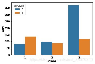
pclass_sur=text.groupby(['Pclass'])['Survived'].value_counts()

import seaborn as sns
sns.countplot(x='Pclass',hue='Survived',data=text)

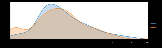
facet=sns.FacetGrid(text,hue="Survived",aspect=3)
facet.map(sns.kdeplot,'Age',shade=True)
facet.set(xlim=(0,text['Age'].max()))
facet.add_legend()

 

6.模型建立和评估

 之前已经对数据信息有了基本了解，并进行了探索性分析和数据重构，还对数据进行了可视化分析。那么接下来我们需要将之前的工作集中运用到模型建立中。模型建立和评估包括特征工程、模型搭建、模型评估三部分，其中特征构成对应着数据重构，这部分内容中，我们主要对数据进行缺失值填充、编码分类变量；模型搭建中将切割数据集为训练集和测试集，切割的方法有按比例切割，一般测试集的比例有30%、25%、20%、15%、10% ；按目标变量分层进行等比切割；设置随机种子以便结果能复现。切割数据集是为了后续能评估模型泛化能力。

sklearn之train_test_split()函数各参数含义

X_train,X_test, y_train, y_test =sklearn.model_selection.train_test_split(train_data,train_target,test_size=0.4, random_state=0,stratify=y_train)

train_data：所要划分的样本特征集

train_target：所要划分的样本结果

test_size：样本占比,可以为浮点、整数或None，默认为None

• ①若为浮点时，表示测试集占总样本的百分比

• ②若为整数时，表示测试样本样本数

• ③若为None时，test size自动设置成0.25

train_size：可以为浮点、整数或None，默认为None

• ①若为浮点时，表示训练集占总样本的百分比

• ②若为整数时，表示训练样本的样本数

• ③若为None时，train_size自动被设置成0.75

random_state：可以为整数、RandomState实例或None，默认为None

• ①若为None时，每次生成的数据都是随机，可能不一样

• ②若为整数时，每次生成的数据都相同

stratify：可以为类似数组或None

• ①若为None时，划分出来的测试集或训练集中，其类标签的比例也是随机的

• ②若不为None时，划分出来的测试集或训练集中，其类标签的比例同输入的数组中类标签的比例相同，可以用于处理不均衡的数据集

简单来说， random_state保证了每次得到一样的随机数，stratify保证了training集和testing集的类的比例与原来的比例一致
#https://www.cnblogs.com/Yanjy-OnlyOne/p/11288098.html

【思考】

• 什么情况下切割数据集的时候不用进行随机选取

#思考回答
在数据集本身已经是随机处理之后的，或者说数据集非常大，内部已经足够随机了

      

train = pd.read_csv('train.csv')
train.head()


	PassengerId	Survived	Pclass	Name	Sex	Age	SibSp	Parch	Ticket	Fare	Cabin	Embarked
0	1	0	3	Braund, Mr. Owen Harris	male	22.0	1	0	A/5 21171	7.2500	NaN	S
1	2	1	1	Cumings, Mrs. John Bradley (Florence Briggs Th...	female	38.0	1	0	PC 17599	71.2833	C85	C
2	3	1	3	Heikkinen, Miss. Laina	female	26.0	0	0	STON/O2. 3101282	7.9250	NaN	S
3	4	1	1	Futrelle, Mrs. Jacques Heath (Lily May Peel)	female	35.0	1	0	113803	53.1000	C123	S
4	5	0	3	Allen, Mr. William Henry	male	35.0	0	0	373450	8.0500	NaN	S

6.1缺失值填充

• 对分类变量缺失值：填充某个缺失值字符(NA)、用最多类别的进行填充
• 对连续变量缺失值：填充均值、中位数、众数

使用fillna函数

# 对分类变量进行填充
train['Cabin'] = train['Cabin'].fillna('NA')
train['Embarked'] = train['Embarked'].fillna('S')

# 对连续变量进行填充
train['Age'] = train['Age'].fillna(train['Age'].mean())

6.2编码分类变量

 # 取出所有的输入特征
data = train[['Pclass','Sex','Age','SibSp','Parch','Fare', 'Embarked']]

# 进行虚拟变量转换
data = pd.get_dummies(data)

data.head()


Pclass	Age	SibSp	Parch	Fare	Sex_female	Sex_male	Embarked_C	Embarked_Q	Embarked_S
0	3	22.0	1	0	7.2500	0	1	0	0	1
1	1	38.0	1	0	71.2833	1	0	1	0	0
2	3	26.0	0	0	7.9250	1	0	0	0	1
3	1	35.0	1	0	53.1000	1	0	0	0	1
4	3	35.0	0	0	8.0500	0	1	0	0	1

 6.3切割数据集

from sklearn.model_selection import train_test_split

# 一般先取出X和y后再切割，有些情况会使用到未切割的，这时候X和y就可以用
X = data
y = train['Survived']

# 对数据集进行切割
X_train, X_test, y_train, y_test = train_test_split(X, y, stratify=y, random_state=0)

# 查看数据形状
X_train.shape, X_test.shape

6.4模型建立

from sklearn.linear_model import LogisticRegression
from sklearn.ensemble import RandomForestClassifier

# 默认参数逻辑回归模型
lr = LogisticRegression()
lr.fit(X_train, y_train)
# 查看训练集和测试集score值
print("Training set score: {:.2f}".format(lr.score(X_train, y_train)))
print("Testing set score: {:.2f}".format(lr.score(X_test, y_test)))

#Training set score: 0.80
#Testing set score: 0.78

# 调整参数后的逻辑回归模型
lr2 = LogisticRegression(C=100)
lr2.fit(X_train, y_train)     
print("Training set score: {:.2f}".format(lr2.score(X_train, y_train)))
print("Testing set score: {:.2f}".format(lr2.score(X_test, y_test)))

#Training set score: 0.80
#Testing set score: 0.79

# 默认参数的随机森林分类模型
rfc = RandomForestClassifier()
rfc.fit(X_train, y_train)
print("Training set score: {:.2f}".format(rfc.score(X_train, y_train)))
print("Testing set score: {:.2f}".format(rfc.score(X_test, y_test)))

#Training set score: 0.98
#Testing set score: 0.81

# 调整参数后的随机森林分类模型
rfc2 = RandomForestClassifier(n_estimators=100, max_depth=5)
rfc2.fit(X_train, y_train)
print("Training set score: {:.2f}".format(rfc2.score(X_train, y_train)))
print("Testing set score: {:.2f}".format(rfc2.score(X_test, y_test))) 

#Training set score: 0.85
#Testing set score: 0.83

6.5输出模型预测结果

• 输出模型预测分类标签
• 输出不同分类标签的预测概率

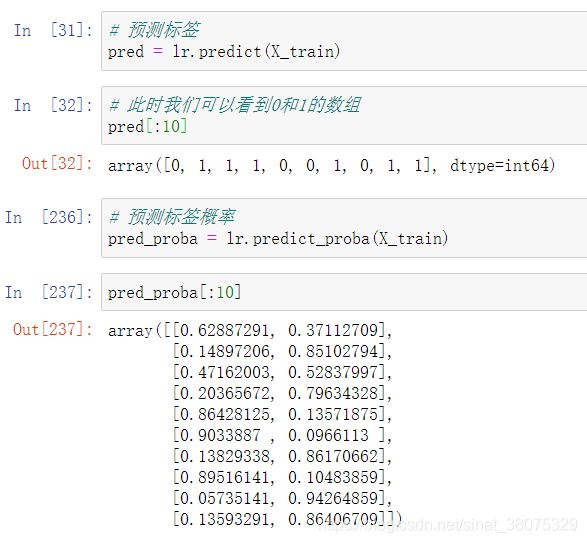
比如此处输出的pred[:10]就是训练集中的前十行数据中每一行数据对应的预测结果，即每一位乘客的存活情况，若存活，则为1，反之为0; pred_proba[:10] 表示前十行数据中每一行数据对应的存活和未存活的概率。

6.6模型评估

• 模型评估是为了知道模型的泛化能力。
• 交叉验证（cross-validation）是一种评估泛化性能的统计学方法，它比单次划分训练集和测试集的方法更加稳定、全面。
• 在交叉验证中，数据被多次划分，并且需要训练多个模型。
• 最常用的交叉验证是 k 折交叉验证（k-fold cross-validation），其中 k 是由用户指定的数字，通常取 5 或 10。
• 准确率（precision）度量的是被预测为正例的样本中有多少是真正的正例
• 召回率（recall）度量的是正类样本中有多少被预测为正类
• f-分数是准确率与召回率的调和平均