MFCC特征提取
For speech/speaker recognition, the most commonly used acoustic features are mel-scale frequency cepstral coefficient (MFCC for short). MFCC takes human perception sensitivity with respect to frequencies into consideration, and therefore are best for speech/speaker recognition. We shall explain the stey-by-step computation of MFCC in this section.
- Pre-emphasis: The speech signal s(n) is sent to a high-pass filter:
s2(n) = s(n) - a*s(n-1)
where s2(n) is the output signal and the value of a is usually between 0.9 and 1.0. The z-transform of the filter isH(z)=1-a*z-1
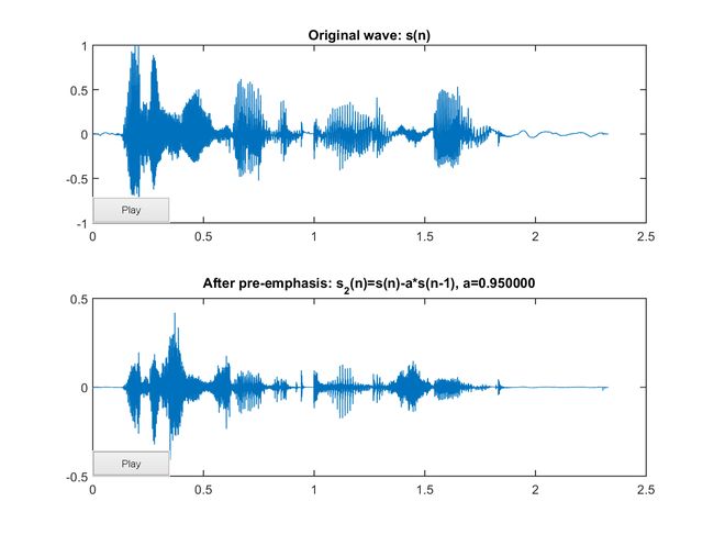
The goal of pre-emphasis is to compensate the high-frequency part that was suppressed during the sound production mechanism of humans. Moreover, it can also amplify the importance of high-frequency formants. The next example demonstrates the effect of pre-emphasis. Example 1: preEmphasis01.mwaveFile='whatFood.wav'; au=myAudioRead(waveFile); y=au.signal; fs=au.fs a=0.95; y2 = filter([1, -a], 1, y); time=(1:length(y))/fs; au2=au; au2.signal=y2; myAudioWrite(au2, 'whatFood_preEmphasis.wav'); subplot(2,1,1); plot(time, y); title('Original wave: s(n)'); subplot(2,1,2); plot(time, y2); title(sprintf('After pre-emphasis: s_2(n)=s(n)-a*s(n-1), a=%f', a)); subplot(2,1,1); set(gca, 'unit', 'pixel'); axisPos=get(gca, 'position'); uicontrol('string', 'Play', 'position', [axisPos(1:2), 60, 20], 'callback', 'sound(y, fs)'); subplot(2,1,2); set(gca, 'unit', 'pixel'); axisPos=get(gca, 'position'); uicontrol('string', 'Play', 'position', [axisPos(1:2), 60, 20], 'callback', 'sound(y2, fs)'); fs = 22050
In the above example, the speech after pre-emphasis sounds sharper with a smaller volume:
- Original: whatFood.wav
- After pre-emphasis: whatFood_preEmphasis.wav
- Frame blocking: The input speech signal is segmented into frames of 20~30 ms with optional overlap of 1/3~1/2 of the frame size. Usually the frame size (in terms of sample points) is equal to power of two in order to facilitate the use of FFT. If this is not the case, we need to do zero padding to the nearest length of power of two. If the sample rate is 16 kHz and the frame size is 320 sample points, then the frame duration is 320/16000 = 0.02 sec = 20 ms. Additional, if the overlap is 160 points, then the frame rate is 16000/(320-160) = 100 frames per second.
- Hamming windowing: Each frame has to be multiplied with a hamming window in order to keep the continuity of the first and the last points in the frame (to be detailed in the next step). If the signal in a frame is denoted by s(n), n = 0,…N-1, then the signal after Hamming windowing is s(n)*w(n), where w(n) is the Hamming window defined by:
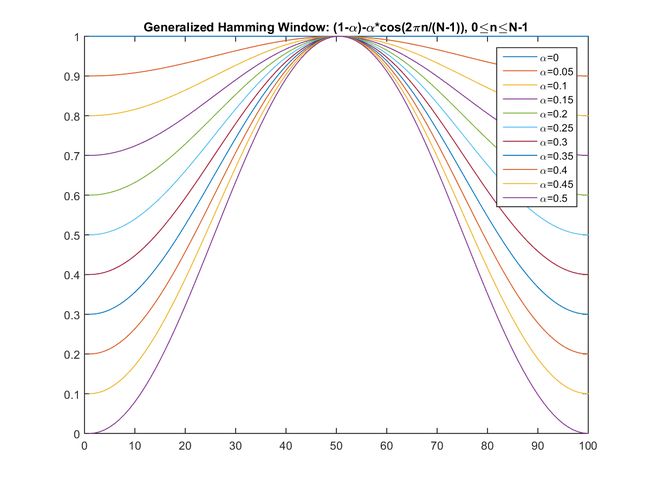
w(n, a) = (1 - a) - a cos(2pn/(N-1)),0≦n≦N-1
Different values of a corresponds to different curves for the Hamming windows shown next: Example 2: hammingWindow01.m% Plot of generalized Hamming windows N=100; n=(0:N-1)'; alpha=linspace(0,0.5,11)'; h=[]; for i=1:length(alpha), h = [h, (1-alpha(i))-alpha(i)*cos(2*pi*n/(N-1))]; end plot(h); title('Generalized Hamming Window: (1-\alpha)-\alpha*cos(2\pin/(N-1)), 0\leqn\leqN-1'); legendStr={}; for i=1:length(alpha), legendStr={legendStr{:}, ['\alpha=', num2str(alpha(i))]}; end legend(legendStr);
In practice, the value of a is set to 0.46. MATLAB also provides the command
hammingfor generating the curve of a Hamming window. - Fast Fourier Transform or FFT: Spectral analysis shows that different timbres in speech signals corresponds to different energy distribution over frequencies. Therefore we usually perform FFT to obtain the magnitude frequency response of each frame.
When we perform FFT on a frame, we assume that the signal within a frame is periodic, and continuous when wrapping around. If this is not the case, we can still perform FFT but the incontinuity at the frame's first and last points is likely to introduce undesirable effects in the frequency response. To deal with this problem, we have two strategies:
- Multiply each frame by a Hamming window to increase its continuity at the first and last points.
- Take a frame of a variable size such that it always contains a integer multiple number of the fundamental periods of the speech signal.

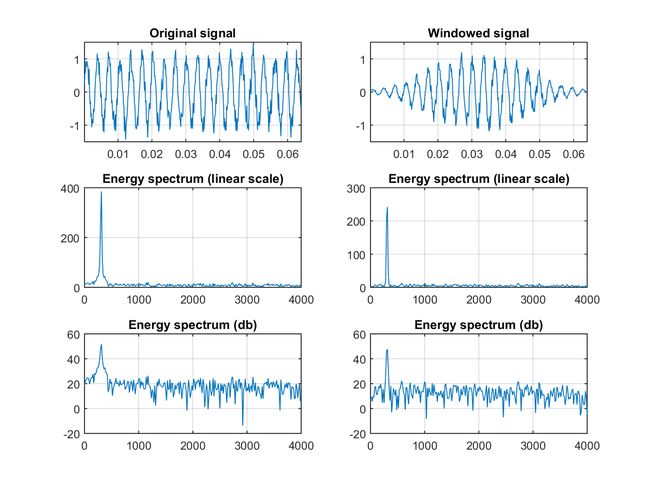
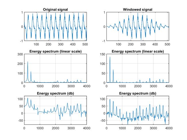
In the above example, the singal is a sinusoidal function plus some noise. Without the use of a Hamming window, the discontinuity at the frame's first and last points will make the peak in the frequency response wider and less obvious. With the use of a Hamming, the peak is sharper and more distinct in the frequency response. The following example uses a speech signal for the same test. Example 4: windowing02.mwaveFile='littleStar.wav'; au=myAudioRead(waveFile); y=au.signal; fs=au.fs; nbits=au.nbits; n=512; t=(1:n)'/fs; startIndex=30418; endIndex=startIndex+n-1; original=y(startIndex:endIndex); windowed=original.*hamming(n); [mag1, phase1, freq1]=fftOneSide(original, fs); [mag2, phase2, freq2]=fftOneSide(windowed, fs); subplot(3,2,1); plot(original); grid on; axis([-inf inf -1 1]); title('Original signal'); subplot(3,2,2); plot(windowed); grid on; axis([-inf inf -1 1]); title('Windowed signal'); subplot(3,2,3); plot(freq1, mag1); grid on; title('Energy spectrum (linear scale)'); subplot(3,2,4); plot(freq2, mag2); grid on; title('Energy spectrum (linear scale)'); subplot(3,2,5); plot(freq1, 20*log(mag1)); grid on; axis([-inf inf -80 120]); title('Energy spectrum (db)'); subplot(3,2,6); plot(freq2, 20*log(mag2)); grid on; axis([-inf inf -80 120]); title('Energy spectrum (db)');
In the above example, we use a frame from a clip of singing voice for the same test. With the use of a Hamming window, the harmonics in the frequency response are much sharper.
Remember that if the input frame consists of 3 identical fundamental periods, then the magnitude frequency response will be inserted 2 zeros between every two neighboring points of the frequency response of a single fundamental periods. (See the chapter on Fourier transform for more details.) In other words, the harmonics of the frequency response is generally caused by the repeating fundamental periods in the frame. However, we are more interested in the envelope of the frequency response instead of the frequency response itself. To extract an envelop-like features, we use the triangular bandpass filters, as explained in the next step.
- Triangular Bandpass Filters: We multiple the magnitude frequency response by a set of 20 triangular bandpass filters to get the log energy of each triangular bandpass filter. The positions of these filters are equally spaced along the Mel frequency, which is related to the common linear frequency f by the following equation:
mel(f)=1125*ln(1+f/700)
Mel-frequency is proportional to the logarithm of the linear frequency, reflecting similar effects in the human's subjective aural perception. The following example plots the relationship between the mel and the linear frequencies: Example 5: showMelFreq01.mlinFreq=0:8000; melFreq=lin2melFreq(linFreq); plot(linFreq, melFreq); xlabel('Frequency'); ylabel('Mel-frequency'); title('Frequency to mel-frequency curve'); axis equal tight
In practice, we have two choices for the triangular bandpass filters, as shown in the next example: Example 6: showTriFilterBank01.mfs=16000; filterNum=20; plotOpt=1; getTriFilterBankPrm(fs, filterNum, plotOpt);
The reasons for using triangular bandpass filters are two fold:- Smooth the magnitude spectrum such that the harmonics are flattened in order to obtain the envelop of the spectrum with harmonics. This indicates that the pitch of a speech signal is generally not presented in MFCC. As a result, a speech recognition system will behave more or less the same when the input utterances are of the same timbre but with different tones/pitch.
- Reduce the size of the features involved.
- Discrete cosine transform or DCT: In this step, we apply DCT on the 20 log energy Ek obtained from the triangular bandpass filters to have L mel-scale cepstral coefficients. The formula for DCT is shown next.
Cm=Sk=1Ncos[m*(k-0.5)*p/N]*Ek, m=1,2, ..., L
where N is the number of triangular bandpass filters, L is the number of mel-scale cepstral coefficients. Usually we set N=20 and L=12. Since we have performed FFT, DCT transforms the frequency domain into a time-like domain called quefrency domain. The obtained features are similar to cepstrum, thus it is referred to as the mel-scale cepstral coefficients, or MFCC. MFCC alone can be used as the feature for speech recognition. For better performance, we can add the log energy and perform delta operation, as explained in the next two steps. - Log energy: The energy within a frame is also an important feature that can be easily obtained. Hence we usually add the log energy as the 13rd feature to MFCC. If necessary, we can add some other features at this step, including pitch, zero cross rate, high-order spectrum momentum, and so on.
- Delta cepstrum: It is also advantagous to have the time derivatives of (energy+MFCC) as new features, which shows the velocity and acceleration of (energy+MFCC). The equations to compute these features are:
△Cm(t) = [St=-MMCm(t+t)t] / [St=-MMt2]
The value of M is usually set to 2. If we add the velocity, the feature dimension is 26. If we add both the velocity and the acceleration, the feature dimension is 39. Most of the speech recognition systems on PC use these 39-dimensional features for recognition.