Convolutional Neural Networks编程(week 1)
(一)Convolutional Neural Networks: step by step
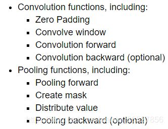
一、步骤
二、Convolutional Neural Networks
1.Zero-Padding
def zero_pad(X, pad):
X_pad = np.pad(X, ((0,0), (pad,pad), (pad,pad), (0,0)), 'constant', constant_values = (pad,pad))
return X_pad
plt.subplots函数
2.Single step of convolution
def conv_single_step(a_slice_prev, W, b):
s = np.multiply(a_slice_prev,W)
Z =np.sum(s)
Z = Z+b
return Z
3.Convolutional Neural Networks - Forward pass
def conv_forward(A_prev, W, b, hparameters):
(m, n_H_prev, n_W_prev, n_C_prev) = A_prev.shape
(f, f, n_C_prev, n_C) = W.shape
stride = hparameters["stride"]
pad = hparameters["pad"]
n_H =int((n_H_prev+2*pad-f)/stride)+1
n_W =int((n_W_prev+2*pad-f)/stride)+1
Z = np.zeros((m, n_H, n_W, n_C))
A_prev_pad = zero_pad(A_prev, pad)
for i in range(m): # loop over the batch of training examples
a_prev_pad = A_prev_pad[i,:,:,:] # Select ith training example's padded activation
for h in range(n_H): # loop over vertical axis of the output volume
for w in range(n_W): # loop over horizontal axis of the output volume
for c in range(n_C): # loop over channels (= #filters) of the output volume
# Find the corners of the current "slice" (≈4 lines)
vert_start = stride * h
vert_end = vert_start + f
horiz_start = stride * w
horiz_end = horiz_start + f
# Use the corners to define the (3D) slice of a_prev_pad (See Hint above the cell). (≈1 line)
a_slice_prev = a_prev_pad[ vert_start: vert_end,horiz_start:horiz_end,:]
# Convolve the (3D) slice with the correct filter W and bias b, to get back one output neuron. (≈1 line)
Z[i, h, w, c] = conv_single_step(a_slice_prev,W[:,:,:,c], b[:,:,:,c])
assert(Z.shape == (m, n_H, n_W, n_C))
cache = (A_prev, W, b, hparameters)
return Z, cache
4.Pooling layer
def pool_forward(A_prev, hparameters, mode = "max"):
(m, n_H_prev, n_W_prev, n_C_prev) = A_prev.shape
f = hparameters["f"]
stride = hparameters["stride"]
n_H = int(1 + (n_H_prev - f) / stride)
n_W = int(1 + (n_W_prev - f) / stride)
n_C = n_C_prev
A = np.zeros((m, n_H, n_W, n_C))
for i in range(m): # loop over the training examples
for h in range(n_H): # loop on the vertical axis of the output volume
for w in range(n_W): # loop on the horizontal axis of the output volume
for c in range (n_C): # loop over the channels of the output volume
# Find the corners of the current "slice" (≈4 lines)
vert_start = h*stride
vert_end = vert_start+f
horiz_start = w*stride
horiz_end = horiz_start+f
# Use the corners to define the current slice on the ith training example of A_prev, channel c. (≈1 line)
a_prev_slice = A_prev[i, vert_start:vert_end, horiz_start:horiz_end, c]
# Compute the pooling operation on the slice. Use an if statment to differentiate the modes. Use np.max/np.mean.
if mode == "max":
A[i, h, w, c] = np.max(a_prev_slice)
elif mode == "average":
A[i, h, w, c] = np.mean(a_prev_slice)
cache = (A_prev, hparameters)
assert(A.shape == (m, n_H, n_W, n_C))
return A, cache
5.Backpropagation in convolutional neural networks
def conv_backward(dZ, cache):
(A_prev, W, b, hparameters) = cache
(m, n_H_prev, n_W_prev, n_C_prev) = A_prev.shape
(f, f, n_C_prev, n_C) = W.shape
stride = hparameters["stride"]
pad = hparameters["pad"]
# Retrieve dimensions from dZ's shape
(m, n_H, n_W, n_C) = dZ.shape
dA_prev = np.zeros((m, n_H_prev, n_W_prev, n_C_prev))
dW = np.zeros((f, f, n_C_prev, n_C))
db = np.zeros((1, 1, 1, n_C))
A_prev_pad = zero_pad(A_prev, pad)
dA_prev_pad = zero_pad(dA_prev, pad)
for i in range(m): # loop over the training examples
# select ith training example from A_prev_pad and dA_prev_pad
a_prev_pad = A_prev_pad[i,:,:,:]
da_prev_pad = dA_prev_pad[i,:,:,:]
for h in range(n_H): # loop over vertical axis of the output volume
for w in range(n_W): # loop over horizontal axis of the output volume
for c in range(n_C): # loop over the channels of the output volume
# Find the corners of the current "slice"
vert_start = stride * h
vert_end = vert_start + f
horiz_start = stride * w
horiz_end = horiz_start + f
# Use the corners to define the slice from a_prev_pad
a_slice = A_prev_pad[i, vert_start:vert_end, horiz_start:horiz_end, :]
# Update gradients for the window and the filter's parameters using the code formulas given above
da_prev_pad[vert_start:vert_end, horiz_start:horiz_end, :] += W[:,:,:,c] * dZ[i, h, w, c]
dW[:,:,:,c] += a_slice * dZ[i, h, w, c]
db[:,:,:,c] += dZ[i, h, w, c]
# Set the ith training example's dA_prev to the unpaded da_prev_pad (Hint: use X[pad:-pad, pad:-pad, :])
dA_prev[i, :, :, :] = da_prev_pad[pad:-pad, pad:-pad, :]
### END CODE HERE ###
# Making sure your output shape is correct
assert(dA_prev.shape == (m, n_H_prev, n_W_prev, n_C_prev))
return dA_prev, dW, db
6.Pooling layer - backward pass
def create_mask_from_window(x):
mask = (x==np.max(x))
return mask
7.Average pooling - backward pass
def distribute_value(dz, shape):
(n_H, n_W) =shape
average = dz/(n_H*n_W)
a = dz/(n_H*n_W)
return a
8.Putting it together: Pooling backward
def pool_backward(dA, cache, mode = "max"):
(A_prev, hparameters) =cache
stride = hparameters["stride"]
f = hparameters["f"]
m, n_H_prev, n_W_prev, n_C_prev =A_prev.shape
m, n_H, n_W, n_C =dA.shape
dA_prev = np.zeros((m, n_H_prev, n_W_prev, n_C_prev))
for i in range(m): # loop over the training examples
# select training example from A_prev (≈1 line)
a_prev = A_prev[i,:,:,:]
for h in range(n_H): # loop on the vertical axis
for w in range(n_W): # loop on the horizontal axis
for c in range(n_C): # loop over the channels (depth)
# Find the corners of the current "slice" (≈4 lines)
vert_start = stride * h
vert_end = vert_start + f
horiz_start = stride * w
horiz_end = horiz_start + f
# Compute the backward propagation in both modes.
if mode == "max":
# Use the corners and "c" to define the current slice from a_prev (≈1 line)
a_prev_slice = a_prev[vert_start:vert_end, horiz_start:horiz_end, c]
# Create the mask from a_prev_slice (≈1 line)
mask = create_mask_from_window(a_prev_slice)
# Set dA_prev to be dA_prev + (the mask multiplied by the correct entry of dA) (≈1 line)
dA_prev[i, vert_start: vert_end, horiz_start: horiz_end, c] += mask * dA[i, h, w, c]
elif mode == "average":
# Get the value a from dA (≈1 line)
da = dA[i, h, w, c]
# Define the shape of the filter as fxf (≈1 line)
shape = (f,f)
# Distribute it to get the correct slice of dA_prev. i.e. Add the distributed value of da. (≈1 line)
dA_prev[i, vert_start: vert_end, horiz_start: horiz_end, c] += distribute_value(da, shape)
### END CODE ###
# Making sure your output shape is correct
assert(dA_prev.shape == A_prev.shape)
return dA_prev
(二)Convolutional Neural Networks: Application
import math
import numpy as np
import h5py
import matplotlib.pyplot as plt
import scipy
from PIL import Image
from scipy import ndimage
import tensorflow as tf
from tensorflow.python.framework import ops
from cnn_utils import *
%matplotlib inline
np.random.seed(1)
X_train_orig, Y_train_orig, X_test_orig, Y_test_orig, classes = load_dataset()
X_train = X_train_orig/255.
X_test = X_test_orig/255.
Y_train = convert_to_one_hot(Y_train_orig, 6).T
Y_test = convert_to_one_hot(Y_test_orig, 6).T
1.1 - Create placeholders
def create_placeholders(n_H0, n_W0, n_C0, n_y):
"""
Creates the placeholders for the tensorflow session.
Arguments:
n_H0 -- scalar, height of an input image
n_W0 -- scalar, width of an input image
n_C0 -- scalar, number of channels of the input
n_y -- scalar, number of classes
Returns:
X -- placeholder for the data input, of shape [None, n_H0, n_W0, n_C0] and dtype "float"
Y -- placeholder for the input labels, of shape [None, n_y] and dtype "float"
"""
X = tf.placeholder(shape=[None, n_H0, n_W0, n_C0],dtype="float32")
Y = tf.placeholder(shape=[None, n_y],dtype="float32")
return X, Y
1.2 - Initialize parameters
def initialize_parameters():
"""
Initializes weight parameters to build a neural network with tensorflow. The shapes are:
W1 : [4, 4, 3, 8]
W2 : [2, 2, 8, 16]
Returns:
parameters -- a dictionary of tensors containing W1, W2
"""
tf.set_random_seed(1) # so that your "random" numbers match ours
W1 =tf.get_variable("W1", [4, 4, 3, 8], initializer = tf.contrib.layers.xavier_initializer(seed = 0) )
W2 =tf.get_variable("W2", [2, 2, 8, 16], initializer = tf.contrib.layers.xavier_initializer(seed = 0) )
parameters = {"W1": W1,
"W2": W2}
return parameters
1.2 - Forward propagation
def forward_propagation(X, parameters):
"""
Implements the forward propagation for the model:
CONV2D -> RELU -> MAXPOOL -> CONV2D -> RELU -> MAXPOOL -> FLATTEN -> FULLYCONNECTED
Arguments:
X -- input dataset placeholder, of shape (input size, number of examples)
parameters -- python dictionary containing your parameters "W1", "W2"
the shapes are given in initialize_parameters
Returns:
Z3 -- the output of the last LINEAR unit
"""
# Retrieve the parameters from the dictionary "parameters"
W1 = parameters['W1']
W2 = parameters['W2']
# CONV2D: stride of 1, padding 'SAME'
Z1 = tf.nn.conv2d(X,W1,strides=[1,1,1,1],padding="SAME")
# RELU
A1 = tf.nn.relu(Z1)
# MAXPOOL: window 8x8, sride 8, padding 'SAME'
P1 = tf.nn.max_pool(A1,ksize=[1,8,8,1],strides=[1,8,8,1],padding="SAME")
# CONV2D: filters W2, stride 1, padding 'SAME'
Z2 = tf.nn.conv2d(P1,W2,strides=[1,1,1,1],padding="SAME")
# RELU
A2 = tf.nn.relu(Z2)
# MAXPOOL: window 4x4, stride 4, padding 'SAME'
P2 = tf.nn.max_pool(A2,ksize=[1,4,4,1],strides=[1,4,4,1],padding="SAME")
# FLATTEN
P2 = tf.contrib.layers.flatten(P2)
# FULLY-CONNECTED without non-linear activation function (not not call softmax).
# 6 neurons in output layer. Hint: one of the arguments should be "activation_fn=None"
Z3 = tf.contrib.layers.fully_connected(P2,6,activation_fn=None)
return Z3
1.3 - Compute cost
def compute_cost(Z3, Y):
"""
Computes the cost
Arguments:
Z3 -- output of forward propagation (output of the last LINEAR unit), of shape (6, number of examples)
Y -- "true" labels vector placeholder, same shape as Z3
Returns:
cost - Tensor of the cost function
"""
cost = tf.nn.softmax_cross_entropy_with_logits(logits = Z3, labels = Y)
cost=tf.reduce_mean(cost)
return cost
1.4 Model
def model(X_train, Y_train, X_test, Y_test, learning_rate = 0.009,
num_epochs = 100, minibatch_size = 64, print_cost = True):
"""
Implements a three-layer ConvNet in Tensorflow:
CONV2D -> RELU -> MAXPOOL -> CONV2D -> RELU -> MAXPOOL -> FLATTEN -> FULLYCONNECTED
Arguments:
X_train -- training set, of shape (None, 64, 64, 3)
Y_train -- test set, of shape (None, n_y = 6)
X_test -- training set, of shape (None, 64, 64, 3)
Y_test -- test set, of shape (None, n_y = 6)
learning_rate -- learning rate of the optimization
num_epochs -- number of epochs of the optimization loop
minibatch_size -- size of a minibatch
print_cost -- True to print the cost every 100 epochs
Returns:
train_accuracy -- real number, accuracy on the train set (X_train)
test_accuracy -- real number, testing accuracy on the test set (X_test)
parameters -- parameters learnt by the model. They can then be used to predict.
"""
ops.reset_default_graph() # to be able to rerun the model without overwriting tf variables
tf.set_random_seed(1) # to keep results consistent (tensorflow seed)
seed = 3 # to keep results consistent (numpy seed)
(m, n_H0, n_W0, n_C0) = X_train.shape
n_y = Y_train.shape[1]
costs = [] # To keep track of the cost
# Create Placeholders of the correct shape
### START CODE HERE ### (1 line)
X, Y = create_placeholders(n_H0, n_W0, n_C0, n_y)
### END CODE HERE ###
# Initialize parameters
### START CODE HERE ### (1 line)
parameters = initialize_parameters()
### END CODE HERE ###
# Forward propagation: Build the forward propagation in the tensorflow graph
### START CODE HERE ### (1 line)
Z3 = forward_propagation(X, parameters)
### END CODE HERE ###
# Cost function: Add cost function to tensorflow graph
### START CODE HERE ### (1 line)
cost = compute_cost(Z3, Y)
### END CODE HERE ###
# Backpropagation: Define the tensorflow optimizer. Use an AdamOptimizer that minimizes the cost.
### START CODE HERE ### (1 line)
optimizer = tf.train.AdamOptimizer(learning_rate=learning_rate).minimize(cost)
### END CODE HERE ###
# Initialize all the variables globally
init = tf.global_variables_initializer()
# Start the session to compute the tensorflow graph
with tf.Session() as sess:
# Run the initialization
sess.run(init)
# Do the training loop
for epoch in range(num_epochs):
minibatch_cost = 0.
num_minibatches = int(m / minibatch_size) # number of minibatches of size minibatch_size in the train set
seed = seed + 1
minibatches = random_mini_batches(X_train, Y_train, minibatch_size, seed)
for minibatch in minibatches:
# Select a minibatch
(minibatch_X, minibatch_Y) = minibatch
# IMPORTANT: The line that runs the graph on a minibatch.
# Run the session to execute the optimizer and the cost, the feedict should contain a minibatch for (X,Y).
### START CODE HERE ### (1 line)
_ , temp_cost = sess.run([optimizer,cost], feed_dict = {X: minibatch_X, Y: minibatch_Y})
### END CODE HERE ###
minibatch_cost += temp_cost / num_minibatches
# Print the cost every epoch
if print_cost == True and epoch % 5 == 0:
print ("Cost after epoch %i: %f" % (epoch, minibatch_cost))
if print_cost == True and epoch % 1 == 0:
costs.append(minibatch_cost)
# plot the cost
plt.plot(np.squeeze(costs))
plt.ylabel('cost')
plt.xlabel('iterations (per tens)')
plt.title("Learning rate =" + str(learning_rate))
plt.show()
# Calculate the correct predictions
predict_op = tf.argmax(Z3, 1)
correct_prediction = tf.equal(predict_op, tf.argmax(Y, 1))
# Calculate accuracy on the test set
accuracy = tf.reduce_mean(tf.cast(correct_prediction, "float"))
print(accuracy)
train_accuracy = accuracy.eval({X: X_train, Y: Y_train})
test_accuracy = accuracy.eval({X: X_test, Y: Y_test})
print("Train Accuracy:", train_accuracy)
print("Test Accuracy:", test_accuracy)
return train_accuracy, test_accuracy, parameters