车道线滑动窗口及拟合多项式实现

（本内容来自优达学城无人驾驶纳米学位）

准备：

经过“灰度——阈值化——感兴趣区域”后的车道线图片一张

实现代码如下：
代码讲解（按照代码顺序讲解）：
1、导入包，读取准备好的图片
2、定义一个函数：查找车道线像素位置
（1）截取图片下半部分，使用np.sum()实现图片下半部分像素按列相加，得到[1554 1306 1292 … 5091 5097 5347]，即每列像素总和，此时若使用plt.plot(histogram)绘制直方图即可看到哪一列像素和最高点，也即车道线像素点位置所在

（2）创建一个输出图像用来绘制车道线标记以及可视化结果
注意，这里使用了np.dstack(binary_warped, binary_warped, binary_warped)使得原来的单通道图像变成了三通道图像
（3）找到直方图中的中点、两个峰值点（即两条车道线的起点）
（4）设置滑动窗口数量、宽度、重新绘制滑动窗口的条件：最小像素数，同时由窗口数量得到窗口高度
（5）使用np.nonzero()识别单通道图像，返回所有像素值非零像素点位置组成的元组
注意：这里需要弄懂np.nonzero()返回的元组的组成
（6）创建两个变量，用来设置绘制左右滑动窗口位置起点
（7）创建两个空列表，用来接收左右车道像素索引
（8）遍历滑动窗口数，实现滑动窗口的绘制
遍历实现：
设置两个滑动窗口的X范围以及Y范围变量
在可视化图像（三通道）上绘制滑动窗口
识别窗口内x和y中的非零像素（nonzerox与nonzeroy是列表，因为返回的是一维的，所以为nonzero()[0]）
将识别出来的像素数组加入到是上面创建的接收左右车道像素索引的的空列表中
判断窗口中非零像素的大小是否符合重新绘制滑动窗口的条件，符合则更新左右滑动窗口位置起点
连接索引数组(以前是像素列表的列表)
注意：这里left_lane_inds和right_lane_inds均为2维的，使用np.concatenate((a1, a2, …), axis=0)（axis默认为0）后，将列表连接变成一个列表：[82135 82136 82137 … 14619 14620 14621]
提取出左右滑动窗口的像素位置用于返回
3、定义一个函数：拟合车道线
（1）调用函数（查找车道线像素位置）得到左右车道线像素位置：leftx, lefty, rightx, righty, out_img
（2）使用np.polyfit(x,y,2)为左右车道线作二次多项式拟合
（3）生成用于绘图的x和y值
先生成（0-binary_warped.shape[0]-1）的均匀间隔的列表
使用二次多项式拟合出来的线作***_fitx = *_fit[0]*ploty2 + ***_fit[1]*ploty + ***_fit[2]
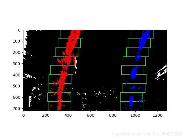
（4）在输出图像上将左右车道线分别染色为红和蓝
（5）在车道线上画出左右多项式
（6）返回输出图像
4、调用拟合车道线函数
5、显示输出图像
至此代码讲解完毕
代码如下：

import numpy as np
import matplotlib.image as mpimg
import matplotlib.pyplot as plt
import cv2

# Load our image
binary_warped = mpimg.imread('warped_example.jpg')

def find_lane_pixels(binary_warped):
    # Take a histogram of the bottom half of the image
    histogram = np.sum(binary_warped[binary_warped.shape[0]//2:,:], axis=0)
    
    # Create an output image to draw on and visualize the result
    out_img = np.dstack((binary_warped, binary_warped, binary_warped))
    
    # Find the peak of the left and right halves of the histogram: starting point for the left and right lines
    midpoint = np.int(histogram.shape[0]//2)
    leftx_base = np.argmax(histogram[:midpoint])
    rightx_base = np.argmax(histogram[midpoint:]) + midpoint

    # Choose the number of sliding windows
    nwindows = 9
    # Set the width of the windows +/- margin
    margin = 100
    # Set minimum number of pixels found to recenter window
    minpix = 50
    # Set height of windows - based on nwindows above and image shape
    window_height = np.int(binary_warped.shape[0]//nwindows)
    
    # Identify the x and y positions of all nonzero pixels in the image
    nonzero = binary_warped.nonzero()
    nonzeroy = np.array(nonzero[0])
    nonzerox = np.array(nonzero[1])
    
    # Current positions to be updated later for each window in nwindows
    leftx_current = leftx_base
    rightx_current = rightx_base
    
    # Create empty lists to receive left and right lane pixel indices
    left_lane_inds = []
    right_lane_inds = []

    # Step through the windows one by one
    for window in range(nwindows):
        # Identify window boundaries in x and y (and right and left)
        win_y_low = binary_warped.shape[0] - (window+1)*window_height
        win_y_high = binary_warped.shape[0] - window*window_height
        win_xleft_low = leftx_current - margin
        win_xleft_high = leftx_current + margin
        win_xright_low = rightx_current - margin
        win_xright_high = rightx_current + margin
        
        # Draw the windows on the visualization image
        cv2.rectangle(out_img,(win_xleft_low,win_y_low),(win_xleft_high,win_y_high),(0,255,0), 2) 
        cv2.rectangle(out_img,(win_xright_low,win_y_low),(win_xright_high,win_y_high),(0,255,0), 2)
        
        # Identify the nonzero pixels in x and y within the window #
        good_left_inds = ((nonzeroy >= win_y_low) & (nonzeroy < win_y_high) & 
        (nonzerox >= win_xleft_low) &  (nonzerox < win_xleft_high)).nonzero()[0]
        good_right_inds = ((nonzeroy >= win_y_low) & (nonzeroy < win_y_high) & 
        (nonzerox >= win_xright_low) &  (nonzerox < win_xright_high)).nonzero()[0]
        
        # Append these indices to the lists
        left_lane_inds.append(good_left_inds)
        right_lane_inds.append(good_right_inds)
        
        # If you found > minpix pixels, recenter next window on their mean position
        if len(good_left_inds) > minpix:
            leftx_current = np.int(np.mean(nonzerox[good_left_inds]))
        if len(good_right_inds) > minpix:        
            rightx_current = np.int(np.mean(nonzerox[good_right_inds]))
            
    # Concatenate the arrays of indices (previously was a list of lists of pixels)
    try:
        left_lane_inds = np.concatenate(left_lane_inds)
        right_lane_inds = np.concatenate(right_lane_inds)
    except ValueError:
        # Avoids an error if the above is not implemented fully
        pass

    # Extract left and right line pixel positions
    leftx = nonzerox[left_lane_inds]
    lefty = nonzeroy[left_lane_inds] 
    rightx = nonzerox[right_lane_inds]
    righty = nonzeroy[right_lane_inds]

    return leftx, lefty, rightx, righty, out_img

def fit_polynomial(binary_warped):
    # Find our lane pixels first
    leftx, lefty, rightx, righty, out_img = find_lane_pixels(binary_warped)

    # Fit a second order polynomial to each using `np.polyfit`
    left_fit = np.polyfit(lefty, leftx, 2)
    right_fit = np.polyfit(righty, rightx, 2)

    # Generate x and y values for plotting
    ploty = np.linspace(0, binary_warped.shape[0]-1, binary_warped.shape[0] )
    try:
        left_fitx = left_fit[0]*ploty**2 + left_fit[1]*ploty + left_fit[2]
        right_fitx = right_fit[0]*ploty**2 + right_fit[1]*ploty + right_fit[2]
    except TypeError:
        # Avoids an error if `left` and `right_fit` are still none or incorrect
        print('The function failed to fit a line!')
        left_fitx = 1*ploty**2 + 1*ploty
        right_fitx = 1*ploty**2 + 1*ploty

    ## Visualization ##
    # Colors in the left and right lane regions
    out_img[lefty, leftx] = [255, 0, 0]
    out_img[righty, rightx] = [0, 0, 255]

    # Plots the left and right polynomials on the lane lines
    plt.plot(left_fitx, ploty, color='yellow')
    plt.show()
    plt.plot(right_fitx, ploty, color='yellow')
    plt.show()

    return out_img

out_img = fit_polynomial(binary_warped)
plt.imshow(out_img)
plt.show()

结果图：



本博客内容不得转载，不得作为他用，仅互相学习，谢谢。