模拟退火算法求函数极值(含MATLAB代码实现)
二、模拟退火算法
1. 简介
模拟退火算法的思想借鉴于固体的退火过程,当固体的温度很高时,内能比较大,固体内的粒子处于快速无序运动状态,当温度慢慢降低,固体的内能减小,粒子逐渐趋于有序,最终固体处于常温状态,内能达到最小,此时粒子最为稳定。
白话理解:一开始为算法设定一个较高的值T(模拟温度),算法不稳定,选择当前较差解的概率很大;随着T的减小,算法趋于稳定,选择较差解的概率减小,最后,T降至终止迭代的条件,得到近似最优解。
2.算法思想及步骤
(1)设置算法的参数:初始温度,结束温度,温度衰减系数,每个温度下的扰动次数,初始状态,初始解
(2)对状态产生扰动,计算新状态下的解,比较两个解的大小,判断是否接受新的状态
(3)在此温度下,对步骤(2)按设置的扰动次数重复进行扰动
(4)对温度进行衰减,并在新的温度下重复(2)(3),直到结束温度
(5)输出记录最优状态和最优解,算法结束
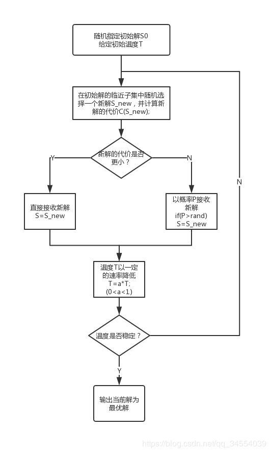
其中,P为算法选择较差解的概率;T 为温度的模拟参数;。
当T很大时,,此时算法以较大概率选择非当前最优解;
P的值随着T的减小而减小;
当时,,此时算法几乎只选择最优解,等同于贪心算法。
%VELASCO, Gimel David F.
%2012-58922
%Cmsc 191
%Simulated Annealing
%Final Exam
%for runs=1:3
clear;
tic;
%%%%%%%%%%%%%%%%%%%%%%%%%%%INPUT ARGUMENTS%%%%%%%Sir Joel, dito po%%%%%%%%%
CostF = 2; % | 1 - DE JONGS | 2 - AXIS PARALLEL HYPER-ELLIPSOID | 3 - ROTATED HYPER-ELLIPSOID | 4 - RASTRIGINS | ow - ACKLEYS |
nVar = 3; %染色体的等位基因数目,染色体长度
VarSize = zeros(nVar);
VarMin = -5.12; %upper bound of variable value
VarMax = 5.12; %lower bound of variable value
MaxIt = 100000;%最大迭代次数
T0 = 100;%初始温度
Tf = 0.000000000000001;%最终温度
alpha = 0.7;%温度下降率
%nPop = 10000;
nMove = 10000;
mu = 0.1;
%sigma = 0.25;
%%
%初始化
test_func = CostF; %sets the number of w/c test function to be solved
ub = VarMax;
lb = VarMin;
ulb = ub; %upper and lower bound
tpl = nVar; %dimensions
x_sol = 2*ulb*(rand(1,tpl)-0.5); %initial guess of the solution x
cooling_ratio = alpha; %sets the cooling ratio to 0.8 i.e. 0.7 < 0.8 < 0.9
num_neigh = nMove; %initializes the size of the random neighbors
cooling_sched = zeros(1); %pre-allocation for speed
cooling_sched(1) = T0; %initializes the cooling schedule T0
iteration_array = zeros(1);
fittest_array = zeros(1);
solution_array = VarSize;
%%%%%%%%%%%%%%%%%%%%%%%%%SIMULATED ANNEALING%%%%%%%%%%%%%%%%%%%%%%%%%%%%%%%
sched = 1; %index
while cooling_sched(sched) > Tf %终止条件
T = cooling_sched(sched); %sets the value of the temperature T
for j=1:num_neigh
r = (cooling_ratio)^sched; %is used so that the randomness of selecting a neighbor becomes narrower
x_tmp = 2*ulb*r*(rand(1,tpl)-0.5); %随机选择一个邻居进行比较
if OBJFUNC(x_tmp,tpl,test_func) < OBJFUNC(x_sol,tpl,test_func) %比较找最优的值
x_sol = x_tmp;
elseif OBJFUNC(x_tmp,tpl,test_func) > OBJFUNC(x_sol,tpl,test_func) %if not, change the solution if it is lucky
delta = OBJFUNC(x_tmp,tpl,test_func) - OBJFUNC(x_sol,tpl,test_func);
p = P(delta,T);
q = rand(1);
if q <= p
x_sol = x_tmp;
end
end
end
fittest_array(sched) = OBJFUNC(x_sol,tpl,test_func);
iteration_array(sched) = sched;
solution_array(sched,:) = x_sol;
cooling_sched(sched+1) = T*(cooling_ratio)^sched;
sched = sched+1;
if sched > MaxIt
break;
end
end
%SOLUTION
if test_func == 1
fprintf('====================DE JONGS FUNCTION=============================\n');
elseif test_func == 2
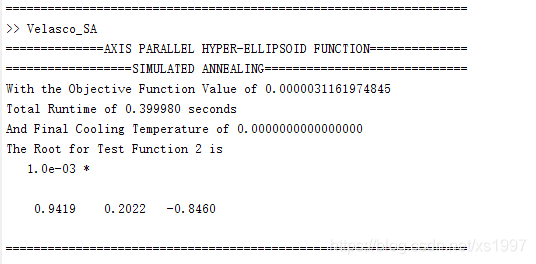
fprintf('==============AXIS PARALLEL HYPER-ELLIPSOID FUNCTION==============\n');
elseif test_func == 3
fprintf('===============ROTATED HYPER-ELLIPSOID FUNCTION====================\n');
elseif test_func == 4
fprintf('====================RASTRIGINS FUNCTION===========================\n');
else
fprintf('=====================ACKLEYS FUNCTION=============================\n');
end
fprintf('==================SIMULATED ANNEALING=============================\n');
fprintf('With the Objective Function Value of %.16f\nTotal Runtime of %f seconds\nAnd Final Cooling Temperature of %.16f\n',OBJFUNC(x_sol,tpl,test_func),toc,cooling_sched(sched));
fprintf('The Root for Test Function %d is\n',test_func);
disp(x_sol)
fprintf('==================================================================\n');
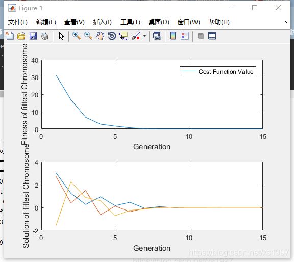
figure
subplot(2,1,1);
plot(iteration_array,fittest_array);
legend('Cost Function Value');
xlabel('Generation');
ylabel('Fitness of fittest Chromosome');
solution_array = transpose(solution_array);
subplot(2,1,2);
plot(iteration_array,solution_array);
xlabel('Generation');
ylabel('Solution of fittest Chromosome');
%end结果: