Kaggle离职员工分析

摘要：使用kaggle公开数据为数据源：员工离职数据，使用Pyecharts分析员工离职情况。针对优秀员工， 使用决策树、随机森林 探索影响员工离职的主要因素 ，结果显示，主要因素为工作年限、员工满意度、月平均工作时长、最近一次评估结果、参与项目数量；又分别使用朴素贝叶斯和SVM模型 预测员工是否离职，其中随机森林预测准确度最高，AUC值可以达到99.05%，SVM模型次之，AUC值为97.43%。 针对最低留存率工作年限的员工，使用逻辑回归模型 分析最低留存率工作年限（第五年）员工离职的主要驱动力 。结果显示，延长平均项目用时、发生事故、近5年获得晋升、加薪以及降低员工满意度能降低员工第五年离职概率。

一、导入数据及数据预处理

import pandas as pd
import numpy as np
import matplotlib.pyplot as plt
import seaborn as sns
plt.rc('font',family='FangSong') # 此语句确保绘图中的中文可以正常显示
import warnings
warnings.filterwarnings('ignore')

df = pd.read_csv('HR_comma_sep.csv')
pd.set_option('display.max_rows',4)
df

	satisfaction_level	last_evaluation	number_project	average_montly_hours	time_spend_company	Work_accident	left	promotion_last_5years	sales	salary
0	0.38	0.53	2	157	3	0	1	0	sales	low
1	0.80	0.86	5	262	6	0	1	0	sales	medium
...	...	...	...	...	...	...	...	...	...	...
14997	0.11	0.96	6	280	4	0	1	0	support	low
14998	0.37	0.52	2	158	3	0	1	0	support	low

14999 rows × 10 columns

df.info()

RangeIndex: 14999 entries, 0 to 14998
Data columns (total 10 columns):
 #   Column                 Non-Null Count  Dtype  
---  ------                 --------------  -----  
 0   satisfaction_level     14999 non-null  float64
 1   last_evaluation        14999 non-null  float64
 2   number_project         14999 non-null  int64  
 3   average_montly_hours   14999 non-null  int64  
 4   time_spend_company     14999 non-null  int64  
 5   Work_accident          14999 non-null  int64  
 6   left                   14999 non-null  int64  
 7   promotion_last_5years  14999 non-null  int64  
 8   sales                  14999 non-null  object 
 9   salary                 14999 non-null  object 
dtypes: float64(2), int64(6), object(2)
memory usage: 1.1+ MB

pd.set_option('display.max_rows',None) # 解决df看不全的问题
df.describe().T

	count	mean	std	min	25%	50%	75%	max
satisfaction_level	14999.0	0.612834	0.248631	0.09	0.44	0.64	0.82	1.0
last_evaluation	14999.0	0.716102	0.171169	0.36	0.56	0.72	0.87	1.0
number_project	14999.0	3.803054	1.232592	2.00	3.00	4.00	5.00	7.0
average_montly_hours	14999.0	201.050337	49.943099	96.00	156.00	200.00	245.00	310.0
time_spend_company	14999.0	3.498233	1.460136	2.00	3.00	3.00	4.00	10.0
Work_accident	14999.0	0.144610	0.351719	0.00	0.00	0.00	0.00	1.0
left	14999.0	0.238083	0.425924	0.00	0.00	0.00	0.00	1.0
promotion_last_5years	14999.0	0.021268	0.144281	0.00	0.00	0.00	0.00	1.0

通过箱线图查看异常值

import seaborn as sns
fig, ax = plt.subplots(1,5, figsize=(12, 2))
sns.boxplot(x=df.columns[0], data=df, ax=ax[0])
sns.boxplot(x=df.columns[1], data=df, ax=ax[1])
sns.boxplot(x=df.columns[2], data=df, ax=ax[2])
sns.boxplot(x=df.columns[3], data=df, ax=ax[3])
sns.boxplot(x=df.columns[4], data=df, ax=ax[4])
plt.show()

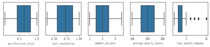
结论： 除了工作年限外, 其他均无异常值。该异常值也反映了该公司员工中以年轻人为主

1. 人力资源总体情况

from pyecharts import options as opts
from pyecharts.charts import Pie

X = [(df.left.value_counts()[1])/(df.shape[0]),(df.left.value_counts()[0])/(df.shape[0])]
X = [round(i,2)  for i in X]
y = ['离职','在职']
c = (
    Pie()
    .add(
        "",
        [list(z) for z in zip(y, X)],
        radius=["30%", "75%"],
    )
    .set_global_opts(
        title_opts=opts.TitleOpts(title="Pie-Radius"),
        legend_opts=opts.LegendOpts(orient="vertical", pos_top="15%", pos_left="2%"),
    )
    .set_series_opts(label_opts=opts.LabelOpts(formatter="{b}: {c}"))
)
c.render_notebook()

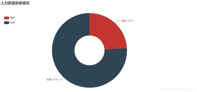
结论： 离职人员占比24%

2. Pyecharts分析是否离职与其余9个因素的关系

2.1 对公司满意度与是否离职的关系

from pyecharts import options as opts
from pyecharts.charts import Boxplot

v1 = [df[df['left']==1]['satisfaction_level'].values.tolist(),df[df['left']==0]['satisfaction_level'].values.tolist()]
c = Boxplot()
c.add_xaxis(['离职','在职'])
c.add_yaxis('对公司满意度',c.prepare_data(v1))
c.set_global_opts(title_opts=opts.TitleOpts(title="对公司满意度与是否离职的关系图"))
c.render_notebook()

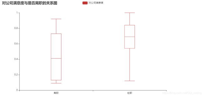
结论： 就中位数而言, 离职人员对公司满意度相对较低, 且离职人员对公司满意度整体波动较大. 另外离职人员中没有满意度为1的评价.

2.2 最新考核评估与是否离职的关系

# 查看具体分箱情况bins
# df4 = df[['last_evaluation','left']]
# pd.cut(df4['last_evaluation'],5,labels= ['低','中低','中','中高','高'],retbins=True)

import pyecharts.options as opts
from pyecharts.charts import Line

df4 = df[['last_evaluation','left']]
df4['last_evaluation'] = pd.cut(df4['last_evaluation'],5,labels= ['低','中低','中','中高','高'])
df4['count'] =1
df_groupby = df4.groupby(by = 'last_evaluation').sum()
df_groupby['left0'] = df_groupby['count'] - df_groupby['left']

c = (
    Line()
    .add_xaxis(df_groupby.index.tolist())
    .add_yaxis("在总体离职员工中的占比", df_groupby['left']/ df_groupby['left'].sum(), is_smooth=True)
    .add_yaxis("在总体在职员工中的占比", df_groupby['left0']/ df_groupby['left0'].sum(), is_smooth=True)
    .set_series_opts(
        areastyle_opts=opts.AreaStyleOpts(opacity=0.5),
        label_opts=opts.LabelOpts(is_show=False),
    )
    .set_global_opts(
        title_opts=opts.TitleOpts(title="最新考核评价与是否离职的关系"),
        xaxis_opts=opts.AxisOpts(
            axistick_opts=opts.AxisTickOpts(is_align_with_label=True),
            is_scale=False,
            boundary_gap=False,
            name="最新考核评价",
        ),
#         yaxis_opts=opts.AxisOpts(name="占比"),
    )
)
c.render_notebook()

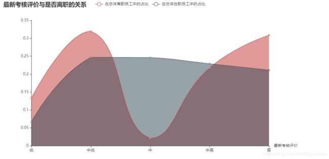
结论：考核评价偏低或偏高的员工更容易离职。在职人员的最新考核评价较为平均，大多数分布在中低-高之间。离职员工的最新考核评价集中在中低和高两个段。

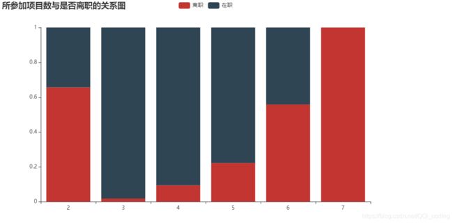
2.3 所参加项目数与是否离职的关系

不同参与项目数的员工离职与在职人员占比分布

from pyecharts import options as opts
from pyecharts.charts import Bar,Pie, Grid

project_left_1 = df[df.left==1].groupby('number_project')['left'].count()
project_all = df.groupby('number_project')['left'].count()
# 分别计算离职人数和在职人数所占比例
project_left1_rate = project_left_1/project_all
project_left0_rate = 1-project_left1_rate


bar = (
    Bar()
    .add_xaxis(project_all.index.tolist())
    .add_yaxis('离职', project_left1_rate.values.reshape(6,).tolist(), stack="stack1")
    .add_yaxis('在职', project_left0_rate.values.reshape(6,).tolist(), stack="stack1")
    .set_series_opts(label_opts=opts.LabelOpts(is_show=False))
    .set_global_opts(title_opts=opts.TitleOpts(title="所参加项目数与是否离职的关系图"))
)

bar.render_notebook()

参与项目数与员工人数及占比分布

c = (
    Pie()
    .add(
        "",
        [list(z) for z in zip(project_all.index.tolist(), project_all.values.reshape(6,).tolist())],
        radius=["20%", "45%"],
    )
    .set_global_opts(
        title_opts=opts.TitleOpts(title="参与项目数与员工人数及占比分布" ,pos_top="10%"),
        legend_opts=opts.LegendOpts(orient="vertical", pos_top="30%", pos_left="5%"),
        
    )
    .set_series_opts(label_opts=opts.LabelOpts(formatter="项目数为{b}的人数: {c} \n 占比：{d}%"))
)

c.render_notebook()

2.4 平均每月工作时长与是否离职的关系

# 平均每月工作时长分段处理，分别统计离职人员和在职人员数量
df_count = df[['average_montly_hours','left']]
df_count['left1'] = [1 if i==1 else 0 for i in df_count['left']]
df_count['left0'] = [1 if i==0 else 0 for i in df_count['left']]

# 分段
bins =[i for i in range(95,315,10)]
df_cut = pd.cut(df_count['average_montly_hours'],bins =bins)
df_count['df_cut'] = df_cut
# 计数
df_cut_count = df_count.groupby(by = 'df_cut').sum()
df_cut_left1_count = df_cut_count['left1'].values.tolist() # 离职人员数量
df_cut_left0_count = df_cut_count['left0'].values.tolist() # 在职人员数量

df_cut_count = df_cut_count.reset_index()
X = [str(i) for i in df_cut_count['df_cut'].values]

from pyecharts import options as opts
from pyecharts.charts import Bar
from pyecharts.faker import Faker
df_average_montly_hours = pd.cut(df[df.left ==1]['average_montly_hours'],bins = 20)
df[df.left ==1]['average_montly_hours'].values.tolist()
c = (
    Bar()
    .add_xaxis(X)
    .add_yaxis("离职",df_cut_left1_count, color=Faker.rand_color())
    .add_yaxis("在职",df_cut_left0_count)
    .set_global_opts(
        title_opts=opts.TitleOpts(title="平均每月工作时长与是否离职的关系"),
        datazoom_opts=[opts.DataZoomOpts(), opts.DataZoomOpts(type_="inside")],
    )
)
c.render_notebook()

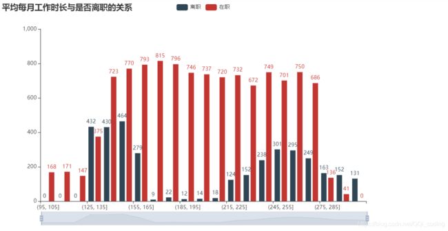
结论： 离职员工的平均每月工作时长集中在(125,165]小时和(215,285]小时之间，而在职员工平均每月工作时长分布均匀，说明平均每月工作时长太短（日均6-7.5h）或太长(日均10h以上)，都可能导致员工离职。将员工月平均工作时长调整在(155,235]之间，

2.5 意外事故和是否离职的关系

accident_df= df[['Work_accident','left','satisfaction_level','last_evaluation','number_project','average_montly_hours'
                ,'salary','time_spend_company']]
accident_df['count']=1
# accident_df.head()

def f(x):
    d = {
     }
    d['count_sum'] = x['count'].sum()
    d['left_sum'] = x['left'].sum()
    d['left_rate'] = (x['left'].sum())/(x['count'].sum())
    d['saf_lvl_mean'] = x['satisfaction_level'].mean()
    d['la_eval_mean'] = x['last_evaluation'].mean()
    d['num_pro_mean'] = x['number_project'].mean()
    d['avg_mh_mean'] = x['average_montly_hours'].mean()
    d['sal_mean'] = x['salary'].mode()
    d['tisp_comp_mean'] = x['time_spend_company'].mean()
    return pd.Series(d, index=['count_sum','left_sum','left_rate', 'saf_lvl_mean', 'la_eval_mean', 'num_pro_mean',
                              'avg_mh_mean','sal_mean','tisp_comp_mean'])

# 查看出过事故的员工和没有出过事故的员工的差别
accident_count = accident_df.groupby(by = 'Work_accident').apply(f)
accident_count

	count_sum	left_sum	left_rate	saf_lvl_mean	la_eval_mean	num_pro_mean	avg_mh_mean	sal_mean	tisp_comp_mean
Work_accident
0	12830	3402	0.265160	0.606833	0.716602	3.805456	201.258613	0 low dtype: object	3.496960
1	2169	169	0.077916	0.648326	0.713144	3.788843	199.818349	0 low dtype: object	3.505763

结论： 出过事故的员工离职率低，为7.8%；没有出过事故的员工离职率高，为26.5%。

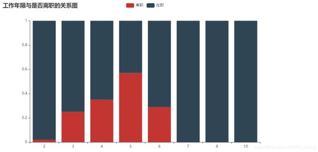
2.6 工作年限与是否离职的关系

from pyecharts import options as opts
from pyecharts.charts import EffectScatter
from pyecharts.globals import SymbolType

# 计算离职人数和在职人数
time_left_1 = df[df.left==1].groupby('time_spend_company')['left'].count()
time_left_0 = df[df.left==0].groupby('time_spend_company')['left'].count()
time_all = df.groupby('time_spend_company')['left'].count()
y_stay_num = time_left_0.values.tolist()
y_left_num = time_left_1.values.tolist()

# 分别计算离职人数和在职人数所占比例
time_left_1_rate = time_left_1/time_all
time_left_1_rate = time_left_1_rate.fillna(0)
time_left_1_rate = time_left_1_rate.map(lambda x: round(x,2))
y_left_rate = time_left_1_rate.values.tolist()

# 调整X轴标签格式
x = time_left_1_rate.index.tolist()
x_data =[str(i) for i in x] # 转化为字符串格式,作为x轴,否则会错位

bar = (
    Bar(init_opts=opts.InitOpts(width="1000px", height="500px"))
    .add_xaxis(xaxis_data=x_data)
    .add_yaxis(
        series_name="离职人数",
        yaxis_data=y_left_num,
        label_opts=opts.LabelOpts(is_show=True),
    )
    .add_yaxis(
        series_name="在职人数",
        yaxis_data=y_stay_num,
        label_opts=opts.LabelOpts(is_show=False),
    )
    .extend_axis(
        yaxis=opts.AxisOpts(
            name="离职率",
            type_="value",
            min_=0,
            max_=0.7,
            interval=0.1,
            axislabel_opts=opts.LabelOpts(formatter="{value} "),
        )
    )
    .set_global_opts(
        title_opts=opts.TitleOpts(title="工作年限与是否离职的关系"),
        tooltip_opts=opts.TooltipOpts(
            is_show=True, trigger="axis", axis_pointer_type="cross"
        ),
        xaxis_opts=opts.AxisOpts(
            type_="category",
            axispointer_opts=opts.AxisPointerOpts(is_show=True, type_="shadow"),
            splitline_opts=opts.SplitLineOpts(is_show=True),
        ),
        yaxis_opts=opts.AxisOpts(
#             name="人数",
            type_="value",
            min_=0,
            max_=5000,
            interval=500,
            axislabel_opts=opts.LabelOpts(formatter="{value}"),
            axistick_opts=opts.AxisTickOpts(is_show=True),
#             splitline_opts=opts.SplitLineOpts(is_show=True),
        ),
    )
)

line = (
    Line()
    .add_xaxis(x_data)
    .add_yaxis(
        series_name="离职率",
        yaxis_index=1,
        y_axis= y_left_rate,
        label_opts=opts.LabelOpts(is_show=True),
    )
)
    
bar.overlap(line).render_notebook()

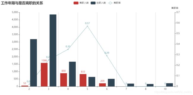
结论： 第五年离职率最高，占比高达57%。其次是第四年、第六年、第三年。工作年限七年及以上离职率为0。

2.7 职务与离职人数、离职率的关系

from pyecharts import options as opts
from pyecharts.charts import Bar, Grid, Line

# 绘制hr数据各个职位的人数的条形图
sales_left_1 = df[df.left==1].groupby('sales')['left'].count()
sales_left_0 = df[df.left==0].groupby('sales')['left'].count()
sales_all = df.groupby('sales')['left'].count()
# 分别计算离职人数和在职人数所占比例
sales_left_1_rate = sales_left_1/sales_all
sales_left_0_rate = 1-sales_left_1_rate
y1_per = [round(i,2) for i in sales_left_1_rate.values.reshape(10,).tolist()]
y1 = []
for i in range(10):
    ha = {
     'value':sales_left_1.values.tolist()[i],'percent':y1_per[i]}
    y1.append(ha)

y0_per = [round(i,2) for i in sales_left_0_rate.values.reshape(10,).tolist()]
y0 = []
for i in range(10):
    ha = {
     'value':sales_left_0.values.tolist()[i],'percent':y0_per[i]}
    y0.append(ha)

x = sales_all.index.tolist()

import pyecharts.options as opts
from pyecharts.charts import Bar, Line
from pyecharts.commons.utils import JsCode
from pyecharts.globals import ThemeType


bar = (
    Bar(init_opts=opts.InitOpts(width="1000px", height="500px"))
    .add_xaxis(x)
    .add_yaxis("离职人数", y1, stack="stack1", category_gap="20%", label_opts=opts.LabelOpts(is_show=False),)
    .add_yaxis("在职人数", y0, stack="stack1", category_gap="50%", label_opts=opts.LabelOpts(is_show=False),)
    .extend_axis(
        yaxis=opts.AxisOpts(
            name="离职率",
            type_="value",
            min_=0,
            max_=0.3,
            interval=0.1,
            axislabel_opts=opts.LabelOpts(formatter="{value}"),
        )
    )
    .set_series_opts(
        label_opts=opts.LabelOpts(
            position="right",
#             formatter=JsCode(
#                 "function(x){return Number(x.data.percent * 100).toFixed() + '%';}"
#             ),
        )
    )
    .set_global_opts(
        title_opts=opts.TitleOpts(title="职务与是否离职的关系"),
        tooltip_opts=opts.TooltipOpts(
            is_show=True, trigger="axis", axis_pointer_type="cross"
        ),
        xaxis_opts=opts.AxisOpts(
            type_="category",
            axispointer_opts=opts.AxisPointerOpts(is_show=True, type_="shadow"),
            axislabel_opts=opts.LabelOpts(rotate=-15),  # 解决x轴名字过长的问题
        ),
        yaxis_opts=opts.AxisOpts(
#             name="人数",
            type_="value",
            min_=0,
            max_=6000,
            interval=1000,
            axislabel_opts=opts.LabelOpts(formatter="{value}"),
            axistick_opts=opts.AxisTickOpts(is_show=True),
            splitline_opts=opts.SplitLineOpts(is_show=True),
        ),
    )
)

scatter = (
    EffectScatter()
    .add_xaxis(x)
    .add_yaxis(series_name = "离职率",
               yaxis_index=1,
               y_axis=[round(i,2) for i in sales_left_1_rate.values.tolist()],
               symbol=SymbolType.ARROW,
               label_opts=opts.LabelOpts(is_show=True),
              )
#     .set_global_opts(title_opts=opts.TitleOpts(title="EffectScatter-不同Symbol"),
#                      xaxis_opts=opts.AxisOpts(splitline_opts=opts.SplitLineOpts(is_show=True)),
#                      yaxis_opts=opts.AxisOpts(splitline_opts=opts.SplitLineOpts(is_show=True)),
#                     )    
)


bar.overlap(scatter).render_notebook()

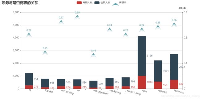
结论：
（1）离职总人数从高到底排名前四的部门为：销售、技术、支持、IT。
（2）hr部门离职率最高，为29%，其他部门离职率在21%-26%之间 。
科研和管理部门离职率比其他序列明显较低，仅为15%左右。

2.8 薪资与是否离职的关系

from pyecharts import options as opts
from pyecharts.charts import Bar

df4 = df[['salary','left']]

c = (
    Bar()
    .add_xaxis(['high','medium','low'])
    .add_yaxis("离职人数", left_1, gap="0%")
    .add_yaxis("在职人数", left_0, gap="0%")
    .set_global_opts(title_opts=opts.TitleOpts(title="薪资与是否离职的关系"))
)

c.render_notebook()

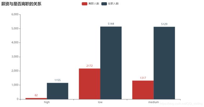
结论： 薪资越高，离职人数越少，离职率越低。其中低薪的员工离职比率最大。故，提高薪水能有效减少离职人数，降低离职率。

2.9 不同薪资和月平均工作时长-与离职率的关系

# sns 绘制热力图
import matplotlib.pyplot as plt
import seaborn as sns
sns.set()
plt.rcParams['font.sans-serif'] = 'Microsoft YaHei'

# 数据
sub_df = df[["salary", "average_montly_hours",'left']]
sub_df['average_montly_hours'] = pd.qcut(sub_df['average_montly_hours'],3,labels= ['短','中','长'])
sub_df['count'] =1

# 绘制热力图
f, (ax1,ax2,ax3) = plt.subplots(figsize=(8, 15),nrows=3)
flights1 = pd.pivot_table(data=sub_df,index = ['salary'],columns = ['average_montly_hours'],values = ['count'],aggfunc = [np.sum])
sns.heatmap(flights1, annot=True, fmt="d", linewidths=.5, ax=ax1)
ax1.set_xlabel('')
ax1.set_title('全部员工薪资和月平均工作时长的分布',fontsize = 15)

flights2 = pd.pivot_table(data=sub_df,index = ['salary'],columns = ['average_montly_hours'],values = ['left'],aggfunc = [np.sum])
sns.heatmap(flights2, annot=True, fmt="d", linewidths=.5, ax=ax2)
ax2.set_xlabel('')
ax2.set_title('离职员工薪资和月平均工作时长的分布',fontsize = 15)

# sub_df['rate'] =
left_rate = flights2.values/flights1.values
sns.heatmap(left_rate*100, annot=True, fmt=".2f", linewidths=.5, ax=ax3)
ax3.set_title('不同薪资和月平均工作时长的员工离职率分布',fontsize = 15)
ax3.set_xlabel('月平均工作时长')
ax3.set_ylabel('薪资水平')
ax3.set_xticklabels(['短','中','长'])
ax3.set_yticklabels(['high','low','medium'])

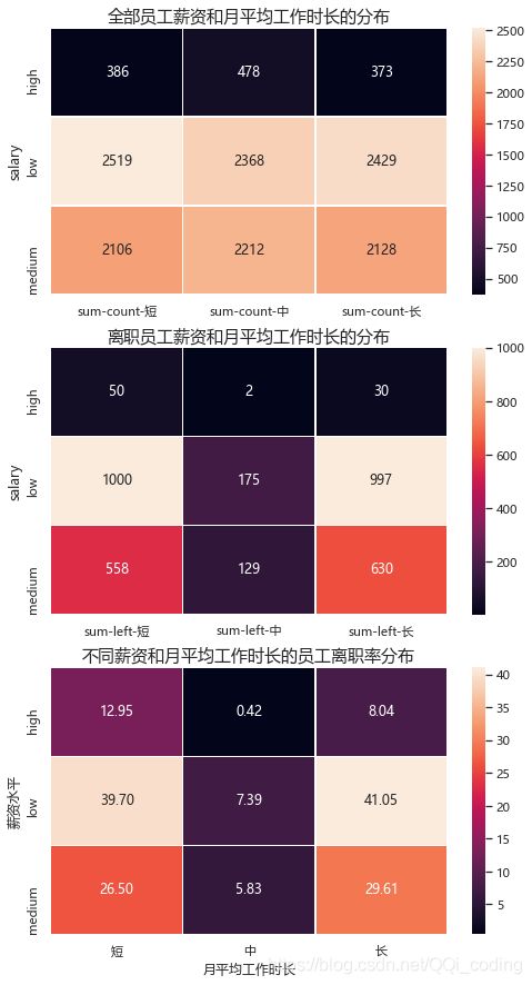
结论：
（1）离职员工集中在（月平均工作时长短&低薪人群）和（月平均工作时长长&低薪人群）。
（2）增加薪水有利于降低离职率，月平均工作时长向中等协调（(168.0, 232.0]）有利于降低离职率。

二、探索影响员工离职的驱动力分析

1. 优秀员工离职驱动力分析

人员流动是市场经济必然现象，但是优秀员工的损失对企业长期价值有严重的影响，人才的持续流失甚至导致企业生命的枯竭。
探索优秀员工离职的主要驱动力，并集中资源避免此类员工的流失具有人才战略意义。
首先我们定义优秀员工：最新考核评估>=0.8 | 参加项目数>=5 | 平均每月工作时长>=230小时
为了尽可能将各个职务，各个工作年限的员工包括进来，三个条件满足任一条件即可

df_excellent = df[(df['last_evaluation']>=0.8)|(df['number_project']>=5)|(df['average_montly_hours']>=230)
                 |(df['time_spend_company']>=4)]
df_excellent.head()
df_excellent.info()

Int64Index: 10372 entries, 1 to 14997
Data columns (total 10 columns):
 #   Column                 Non-Null Count  Dtype  
---  ------                 --------------  -----  
 0   satisfaction_level     10372 non-null  float64
 1   last_evaluation        10372 non-null  float64
 2   number_project         10372 non-null  int64  
 3   average_montly_hours   10372 non-null  int64  
 4   time_spend_company     10372 non-null  int64  
 5   Work_accident          10372 non-null  int64  
 6   left                   10372 non-null  int64  
 7   promotion_last_5years  10372 non-null  int64  
 8   sales                  10372 non-null  object 
 9   salary                 10372 non-null  object 
dtypes: float64(2), int64(6), object(2)
memory usage: 891.3+ KB

# 获取数据
df_dtree = df_excellent.copy()

df_dtree = pd.get_dummies(data = df_dtree,columns=['sales','salary'],drop_first=False)  # 哑变量转换
df_dtree.head()

# 切分自变量和因变量
X = df_dtree.drop(['left'], axis=1) 
y = df_dtree['left']

# 70%为测试集,30%为训练集
from sklearn.model_selection import train_test_split
X_train, X_test, y_train, y_test = train_test_split(X, y, test_size=0.3, random_state=1)

1. 决策树、随机森林分析

from sklearn.model_selection import cross_val_score
from sklearn import datasets
from sklearn.datasets import make_blobs
from sklearn.ensemble import RandomForestClassifier  # 随机森林
from sklearn.tree import DecisionTreeClassifier  # 决策树
from sklearn import tree
from IPython.display import Image  
import graphviz 
import pydotplus
import os
import math
os.environ["PATH"] += os.pathsep + 'G:/program_files/graphviz/bin'

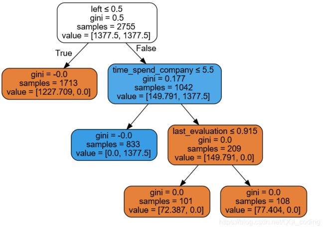
1.1 决策树

超参数选择：考虑到离职人数占比少，存在样本不均衡的现象，故选择class_weight = ‘balanced’，改善样本不均衡带来的预测偏差。

# 决策树实例化
clf = DecisionTreeClassifier(max_depth=5,min_samples_leaf = math.ceil(X.shape[0]*0.07),random_state=0,class_weight = 'balanced')
clf = clf.fit(X_train, y_train)

# 决策树可视化
dot_data = tree.export_graphviz(clf, out_file=None,
                         # 对应特征的名字       
                         feature_names=X_train.columns.values,   
                         filled=True, rounded=True,  
                         special_characters=True)
graph = graphviz.Source(dot_data)
display(graph )

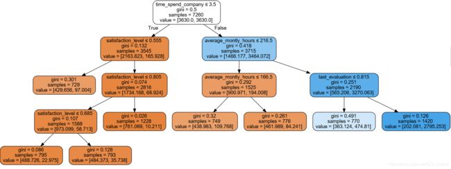
结论: 影响优秀员工离职的主要因素为工作年限、员工满意度、月平均工作时长、最近一次评估结果。

# 对测试集预测
y_pred = clf.predict(X_test)

# 模型检验--混淆矩阵
from sklearn import metrics
from sklearn.metrics import confusion_matrix
from sklearn.metrics import accuracy_score,precision_score,recall_score,f1_score

# 混淆矩阵
conf_df = confusion_matrix(y_test,y_pred,labels = [0,1])

#绘制混淆矩阵
fig= plt.figure(figsize=(10,5))
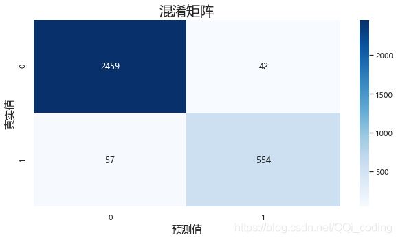
sns.heatmap(conf_df,annot=True,fmt='.20g', cmap=plt.cm.Blues)
plt.title('混淆矩阵',fontsize = 20)
plt.xlabel('预测值',fontsize = 15)
plt.ylabel('真实值',fontsize = 15)
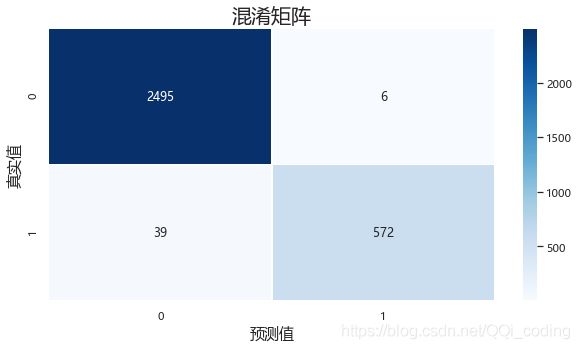
print("决策树模型准确率:" ,'%.2f%%'% (accuracy_score(y_test, y_pred)*100))
print("决策树模型精确率:", '%.2f%%'% (precision_score(y_test, y_pred)*100))
print("决策树模型召回率:", '%.2f%%'% (recall_score(y_test, y_pred)*100))
print("决策树模型F1值:",'%.2f%%'% ( f1_score(y_test, y_pred)*100))

# 5折交叉验证
from  sklearn.model_selection import cross_val_score
clf_accuracy_scores = cross_val_score(clf,X,y,cv=5,scoring = 'accuracy')
print('基于5折交叉验证的决策树模型准确率:',round(clf_accuracy_scores.mean(),2))

决策树模型准确率: 85.31%
决策树模型精确率: 58.33%
决策树模型召回率: 88.22%
决策树模型F1值: 70.23%
基于5折交叉验证的决策树模型准确率: 0.9

结果分析：真实要离职的611人中，预测对了539人，召回率为88.22%；
预测结果显示要离职的924人中，预测对了的为539人，精确率为58.33%。
如果后续需要根据预测结果进行访谈，这样的预测结果会大大增加资源投入，模型效果仍有待改进。

1.2 随机森林

超参数选择 ：因数据类别数量差别很大，使用class_weight = 'balanced’来做平衡，其他使用默认值,查看随机森林分类结果

print(y.value_counts() )
rf0 = RandomForestClassifier(oob_score=True, random_state=10,class_weight = 'balanced')
#  oob_score :即是否采用袋外样本来评估模型的好坏。默认识False。
# 个人推荐设置为True，因为袋外分数反应了一个模型拟合后的泛化能力。

rf0.fit(X_train, y_train)
print(rf0.oob_score_)

y_predprob = rf0.predict_proba(X_test)[:,1] 
print("AUC Score (Train): %f" % metrics.roc_auc_score(y_test, y_predprob))

y_predict = rf0.predict(X_test)
from sklearn.metrics import classification_report
pd.set_option('display.max_rows',None)
print(classification_report(y_test, y_predict))

0    8339
1    2033
Name: left, dtype: int64
0.9858126721763085
AUC Score (Train): 0.990518
              precision    recall  f1-score   support

           0       0.98      1.00      0.99      2501
           1       0.99      0.94      0.96       611

    accuracy                           0.99      3112
   macro avg       0.99      0.97      0.98      3112
weighted avg       0.99      0.99      0.99      3112

​

由结果可以看出： 袋外分数已经很高，而且AUC分数也很高

尝试使用网格搜索交叉验证寻找最佳超参数

#  RandomForestClassifier(oob_score=True, random_state=10,class_weight = 'balanced')

RandomForestClassifier(class_weight='balanced', oob_score=True, random_state=10)

# from sklearn.model_selection import GridSearchCV

# entropy_thresholds = np.linspace(0, 1, 100)
# gini_thresholds = np.linspace(0, 0.2, 100)
# #设置参数矩阵：
# param_grid = [{'criterion': ['entropy'], 'min_impurity_decrease': entropy_thresholds},
#               {'criterion': ['gini'], 'min_impurity_decrease': gini_thresholds},
#               {'max_depth': np.arange(2,10)},
#               {'min_samples_split': np.arange(2,30,2)}]
# rfc = GridSearchCV(RandomForestClassifier(), param_grid, cv=3)
# rfc.fit(X_train, y_train)
# print("best param:{0}\nbest score:{1}".format(rfc.best_params_, rfc.best_score_))

# 预测，绘制混淆矩阵进行检验
# estimator = rfc.best_estimator_
# y_hat = estimator.predict(X_test)
# print(classification_report(y_test,y_hat))

# 计算AUC值进行检验
# y_predprob2 = rf1.predict_proba(X_test)[:,1] 
# print("AUC Score (Train): %f" % metrics.roc_auc_score(y_test, y_predprob2))

优化后和优化前没有明显区别，仍使用原来的模型

模型检验

# ROC曲线和AUC值
from sklearn.metrics import roc_auc_score, auc
import matplotlib.pyplot as plt

y_predict = rf0.predict(X_test)
y_probability = rf0.predict_proba(X_test) #模型的预测得分
fpr, tpr, thresholds = metrics.roc_curve(y_test,y_probability[:,1])
roc_auc = auc(fpr, tpr)  #auc为Roc曲线下的面积

#开始画ROC曲线
plt.plot(fpr, tpr, 'b',label='AUC = %0.2f'% roc_auc)
plt.legend(loc='lower right')
plt.plot([0,1],[0,1],'r--')
plt.xlim([-0.1,1.1])
plt.ylim([-0.1,1.1])
plt.xlabel('False Positive Rate') #横坐标是fpr
plt.ylabel('True Positive Rate')  #纵坐标是tpr
plt.title('Receiver operating characteristic example')
plt.show()
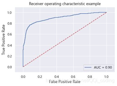
print("随机森林模型的AUC值为：",'%.2f%%'%(roc_auc*100))

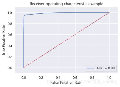
结论： 随机森林模型的AUC值为： 99.05%

# 对测试集预测
y_pred_Randf = rf0.predict(X_test)

# 模型检验--混淆矩阵
from sklearn import metrics
from sklearn.metrics import confusion_matrix
from sklearn.metrics import accuracy_score,precision_score,recall_score,f1_score

# 混淆矩阵
conf_df = confusion_matrix(y_test,y_pred_Randf,labels = [0,1])

#绘制混淆矩阵
fig= plt.figure(figsize=(10,5))
sns.heatmap(conf_df, annot=True, fmt='.20g', linewidths=.5,cmap=plt.cm.Blues)

plt.title('混淆矩阵',fontsize = 20)
plt.xlabel('预测值',fontsize = 15)
plt.ylabel('真实值',fontsize = 15)
print("随机森林模型准确率:" ,'%.2f%%'% (accuracy_score(y_test, y_pred_Randf)*100))
print("随机森林模型精确率:", '%.2f%%'% (precision_score(y_test, y_pred_Randf)*100))
print("随机森林模型召回率:", '%.2f%%'% (recall_score(y_test, y_pred_Randf)*100))
print("随机森林模型F1值:",'%.2f%%'% ( f1_score(y_test, y_pred_Randf)*100))

# 5折交叉验证
from  sklearn.model_selection import cross_val_score
rf0_adj_accuracy_scores = cross_val_score(rf0,X,y,cv=5,scoring = 'accuracy')
print('基于5折交叉验证的随机森林模型准确率:',round(rf0_adj_accuracy_scores.mean(),2))

随机森林模型准确率: 98.55%
随机森林模型精确率: 98.96%
随机森林模型召回率: 93.62%
随机森林模型F1值: 96.22%
基于5折交叉验证的随机森林模型准确率: 0.99

结果分析：真实要离职的611人中，预测对了572人，召回率为93.62%；
预测结果显示要离职的578人中，预测对了的为572人，精确率为98.96%。
相比决策树模型，大大提高了预测的精确度，召回率也由88.22%提升至93.62%，故，随机森林模型预测效果更好。

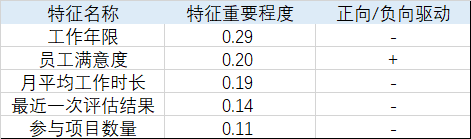
影响员工离职的主要因素

y_importances = rf0.feature_importances_
x_importances = X_train.columns.values
y_pos = np.arange(len(x_importances))
# 横向柱状图
plt.figure(figsize = (10,8))
# plt.barh(y_pos, y_importances, align='center')
sns.barplot(y = x_importances, x= y_importances,orient = 'h')#orient是旋转
plt.yticks(y_pos, x_importances)
plt.xlabel('Importances')
plt.xlim(0,0.3)
plt.title('Features Importances')
plt.show()

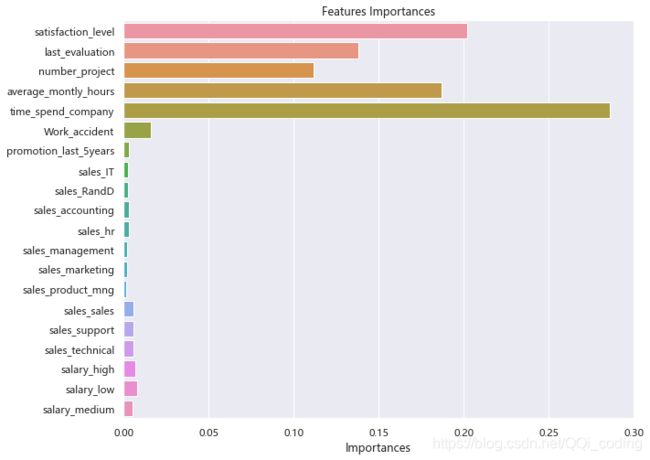
结论： 结果和决策树模型基本相同。影响员工离职的主要因素为，工作年限、员工满意度、月平均工作时长、最近一次评估结果、参与项目数量。

1.2 贝叶斯模型

df3 = df_excellent.copy()
df3 = pd.get_dummies(data = df3,columns=['sales','salary'],drop_first=False)

# 切分变量
X = df3.drop(['left'], axis=1) 
y = df3['left']
X.head()

	satisfaction_level	last_evaluation	number_project	average_montly_hours	time_spend_company	Work_accident	promotion_last_5years	sales_IT	sales_RandD	sales_accounting	sales_hr	sales_management	sales_marketing	sales_product_mng	sales_sales	sales_support	sales_technical	salary_high	salary_low	salary_medium
1	0.80	0.86	5	262	6	0	0	0	0	0	0	0	0	0	1	0	0	0	0	1
2	0.11	0.88	7	272	4	0	0	0	0	0	0	0	0	0	1	0	0	0	0	1
3	0.72	0.87	5	223	5	0	0	0	0	0	0	0	0	0	1	0	0	0	1	0
6	0.10	0.77	6	247	4	0	0	0	0	0	0	0	0	0	1	0	0	0	1	0
7	0.92	0.85	5	259	5	0	0	0	0	0	0	0	0	0	1	0	0	0	1	0

构建模型，进行预测

# splitting X and y into training and testing sets
from sklearn.model_selection import train_test_split
X_train, X_test, y_train, y_test = train_test_split(X, y, test_size=0.4, random_state=1)

# training the model on training set
from sklearn.naive_bayes import GaussianNB
gnb = GaussianNB()
gnb.fit(X_train, y_train)

# making predictions on the testing set
y_pred = gnb.predict(X_test)

模型检验
混淆矩阵-ROC曲线-AUC验证

# comparing actual response values (y_test) with predicted response values (y_pred)
from sklearn import metrics
from sklearn.metrics import confusion_matrix
from sklearn.metrics import accuracy_score,precision_score,recall_score,f1_score

# 混淆矩阵
conf_df = confusion_matrix(y_test,y_pred,labels = [0,1])

#绘制混淆矩阵
fig= plt.figure(figsize=(10,5))
# print(confusion_matrix(y_test, y_pred)) # 输出混淆矩阵数值
sns.heatmap(conf_df,annot=True,fmt='.20g', cmap=plt.cm.Blues)
plt.title('混淆矩阵',fontsize = 20)
plt.xlabel('预测值',fontsize = 15)
plt.ylabel('真实值',fontsize = 15)
print("Gaussian Naive Bayes model 准确率:" ,'%.2f%%'% (accuracy_score(y_test, y_pred)*100))
print("Gaussian Naive Bayes model 精确率:", '%.2f%%'% (precision_score(y_test, y_pred)*100))
print("Gaussian Naive Bayes model 召回率:", '%.2f%%'% (recall_score(y_test, y_pred)*100))
print("Gaussian Naive Bayes model F1值:",'%.2f%%'% ( f1_score(y_test, y_pred)*100))

Gaussian Naive Bayes model 准确率: 83.13%
Gaussian Naive Bayes model 精确率: 54.18%
Gaussian Naive Bayes model 召回率: 82.42%
Gaussian Naive Bayes model F1值: 65.38%

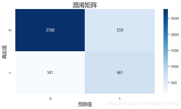
综合对比朴素贝叶斯模型和决策树模型的混淆矩阵，召回率也由88.22%提升至93.62%。

结论： 决策树模型效果更好。

# ROC曲线和AUC值
from sklearn.metrics import roc_auc_score, auc
import matplotlib.pyplot as plt

y_predict = gnb.predict(X_test)
y_probability = gnb.predict_proba(X_test) #模型的预测得分
fpr, tpr, thresholds = metrics.roc_curve(y_test,y_probability[:,1])
roc_auc = auc(fpr, tpr)  #auc为Roc曲线下的面积

#开始画ROC曲线
plt.plot(fpr, tpr, 'b',label='AUC = %0.2f'% roc_auc)
plt.legend(loc='lower right')
plt.plot([0,1],[0,1],'r--')
plt.xlim([-0.1,1.1])
plt.ylim([-0.1,1.1])
plt.xlabel('False Positive Rate') #横坐标是fpr
plt.ylabel('True Positive Rate')  #纵坐标是tpr
plt.title('Receiver operating characteristic example')
plt.show()
print("贝叶斯模型的AUC值为：",'%.2f%%'%(roc_auc*100))

贝叶斯模型的AUC值为： 89.81%

结论： 朴素贝叶斯模型的AUC值小于随机森林的AUC值99.05%。随机森林模型分类效果更好。

交叉验证（5折）

from  sklearn.model_selection import cross_val_score
gnb_accuracy_scores = cross_val_score(gnb,X,y,cv=5,scoring = 'accuracy')
print('基于5折交叉验证的Gaussian Naive Bayes model准确率:',round(gnb_accuracy_scores.mean(),2))

基于5折交叉验证的Gaussian Naive Bayes model准确率: 0.82

结论： 交叉验证结果显示，朴素贝叶斯模型准确率（0.82）低于决策树模型准确率0.9，随机森林模型准确率0.99。

1.3 SVM模型

import numpy as np
import matplotlib.pyplot as plt
from matplotlib.colors import Normalize

from sklearn.svm import SVC
from sklearn.preprocessing import StandardScaler
from sklearn.model_selection import StratifiedShuffleSplit
from sklearn.model_selection import GridSearchCV

# 获取数据
df_svm = df_excellent.copy()
df_svm = pd.get_dummies(data = df_svm,columns=['sales','salary'],drop_first=False)  # 哑变量转换
df_svm.head()

# 切分自变量和因变量
X = df_svm.drop(['left'], axis=1)
y = df_svm['left']

# 70%为测试集,30%为训练集
from sklearn.model_selection import train_test_split
X_train, X_test, y_train, y_test = train_test_split(X, y, test_size=0.3, random_state=1)

scaler = StandardScaler()
X_train_scale = scaler.fit_transform(X_train)
X_test_scale = scaler.transform(X_test)

使用调节好的超参数代入模型中，C=100, gamma=1,class_weight={1: 5}，进行模型实例化。

# 模型实例化
clf_weights = SVC(kernel='rbf',C=100, gamma=1,class_weight={
     1: 5},probability = True) # 不同的内核，差别很大
clf_weights.fit(X_train_scale, y_train)

# 对测试集预测
y_pred = clf_weights.predict(X_test_scale)

模型检验 -ROC曲线-AUC值-混淆矩阵

# ROC曲线和AUC值
from sklearn.metrics import roc_auc_score, auc
import matplotlib.pyplot as plt

y_predict = clf_weights.predict(X_test_scale)
y_probability = clf_weights.predict_proba(X_test_scale) #模型的预测得分
fpr, tpr, thresholds = metrics.roc_curve(y_test,y_probability[:,1])
roc_auc = auc(fpr, tpr)  #auc为Roc曲线下的面积

#开始画ROC曲线
plt.plot(fpr, tpr, 'b',label='AUC = %0.2f'% roc_auc)
plt.legend(loc='lower right')
plt.plot([0,1],[0,1],'r--')
plt.xlim([-0.1,1.1])
plt.ylim([-0.1,1.1])
plt.xlabel('False Positive Rate') #横坐标是fpr
plt.ylabel('True Positive Rate')  #纵坐标是tpr
plt.title('Receiver operating characteristic example')
plt.show()
print("SVM模型的AUC值为：",'%.2f%%'%(roc_auc*100))

SVM模型的AUC值为： 97.43%

# 模型检验--混淆矩阵
from sklearn import metrics
from sklearn.metrics import confusion_matrix
from sklearn.metrics import accuracy_score,precision_score,recall_score,f1_score

# 混淆矩阵
conf_df = confusion_matrix(y_test,y_pred,labels = [0,1])

#绘制混淆矩阵
fig= plt.figure(figsize=(10,5))
sns.heatmap(conf_df,annot=True,fmt='.20g', cmap=plt.cm.Blues)
plt.title('混淆矩阵',fontsize = 20)
plt.xlabel('预测值',fontsize = 15)
plt.ylabel('真实值',fontsize = 15)
print("支持向量机模型准确率:" ,'%.2f%%'% (accuracy_score(y_test, y_pred)*100))
print("支持向量机模型精确率:", '%.2f%%'% (precision_score(y_test, y_pred)*100))
print("支持向量机模型召回率:", '%.2f%%'% (recall_score(y_test, y_pred)*100))
print("支持向量机模型F1值:",'%.2f%%'% ( f1_score(y_test, y_pred)*100))

支持向量机模型准确率: 96.82%
支持向量机模型精确率: 92.95%
支持向量机模型召回率: 90.67%
支持向量机模型F1值: 91.80%

# 5折交叉验证
from  sklearn.model_selection import cross_val_score
clf_accuracy_scores = cross_val_score(clf_weights,X,y,cv=5,scoring = 'accuracy')
print('基于5折交叉验证的决策树模型准确率:',round(clf_accuracy_scores.mean(),2))

基于5折交叉验证的决策树模型准确率: 0.95

调节超参数: C, gamma, class_weight
C, gamma: 实践中，10^-3 至10^3 通常就足够了。如果最佳参数位于网格的边界上，则可以在后续搜索中沿该方向扩展

import numpy as np
import matplotlib.pyplot as plt

from sklearn.svm import SVC
from sklearn.preprocessing import StandardScaler
from sklearn.model_selection import StratifiedShuffleSplit
from sklearn.model_selection import GridSearchCV

C_range = np.logspace(-3,3,7)
gamma_range = np.logspace(-3,3,7)
class_weight_range=[{
     1: 2},{
     1: 5},{
     1: 10},{
     1: 20}]  # 1:5最好
param_grid = dict(gamma=gamma_range, C=C_range,class_weight = [{
     1: 5}]) # 1:5最好
cv = StratifiedShuffleSplit(n_splits=1, test_size=0.3, random_state=42) 
# 数据分为1组，每一组内分训练集和测试集，测试集比例为0.2

grid = GridSearchCV(SVC(), param_grid=param_grid, cv=cv)

# 对标准化后的数据进行训练，寻找最优参数
grid.fit(X_train_scale, y_train)

print("The best parameters are %s with a score of %0.2f"
      % (grid.best_params_, grid.best_score_))
scores = grid.cv_results_['mean_test_score'].reshape(len(C_range),len(gamma_range))
# print(scores)

The best parameters are {'C': 100.0, 'class_weight': {1: 5}, 'gamma': 1.0} with a score of 0.98

# 热力图-直观观察两个参数
class MidpointNormalize(Normalize):

    def __init__(self, vmin=None, vmax=None, midpoint=None, clip=False):
        self.midpoint = midpoint
        Normalize.__init__(self, vmin, vmax, clip)

    def __call__(self, value, clip=None):
        x, y = [self.vmin, self.midpoint, self.vmax], [0, 0.5, 1]
        return np.ma.masked_array(np.interp(value, x, y))

plt.figure(figsize=(8, 6))
plt.subplots_adjust(left=.2, right=0.95, bottom=0.15, top=0.95)
plt.imshow(scores, interpolation='nearest', cmap=plt.cm.hot,
           norm=MidpointNormalize(vmin=0.8, midpoint=0.92))
plt.xlabel('gamma')
plt.ylabel('C')
plt.colorbar()
plt.xticks(np.arange(len(gamma_range)), gamma_range, rotation=45)
plt.yticks(np.arange(len(C_range)), C_range)
plt.title('Validation accuracy')
plt.show()

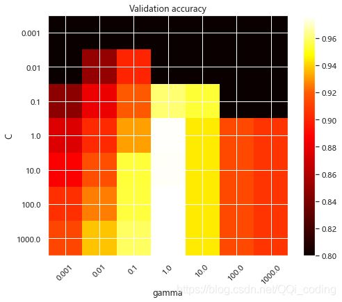
C参数权衡了训练示例的正确分类与决策函数裕度的最大化之间的权衡。对于较大的值 C，如果决策函数可以更好地正确分类所有训练点，则可以接受较小的边距。较低的值C会鼓励较大的余量，因此会简化决策功能，但会降低训练的准确性。换句话说，C在SVM中充当正则化参数。

模型的行为对gamma参数非常敏感。如果 gamma太大，则支持向量的影响区域的半径仅包括支持向量本身，而没有任何正则化C将能够防止过度拟合。

当gamma非常小时，模型过于受限，无法捕获数据的复杂性或“形状”。任何选定的支持向量的影响区域将包括整个训练集。所得模型的行为将类似于带有一组超平面的线性模型，该超平面将两个类别的任何一对的高密度中心分开。

对于中间值，我们可以看到第二个图是不错的机型可以在对角线的发现C和gamma。gamma 通过增加正确分类每个点的重要性（较大的C值），从而提高性能模型的对角线，可以使平滑模型（较低的值）更加复杂。

最后，我们还可以观察到，对于某些中间值，gamma当模型C变得非常大时，我们将获得性能均等的模型：不必通过强制执行较大的余量来进行正则化。RBF内核的半径本身就可以充当良好的结构调整器。在实践中，尽管可能会很有趣的是使用较低的值简化决策函数，C以便支持使用更少内存且预测速度更快的模型。

我们还应注意，分数的微小差异是由交叉验证过程的随机分裂导致的。可以通过增加CV迭代次数来消除那些虚假的变化n_splits，而以计算时间为代价。增加的值数C_range和 gamma_range步骤将增加超参数热图的分辨率。

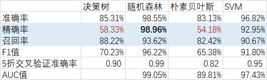
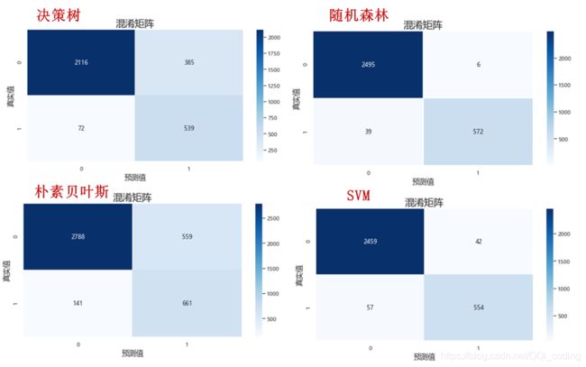
1.4 模型预测效果对比

我们重点关注要离职的员工是否能准确预测出来，以及预测出的要离职的员工是否真的会离职。即，召回率和精确率尽可能接近1，是我们想要的结果。
对比4中模型的预测结果，我们可以看出，随机森林和SVM的结果最好，召回率和精确率都在90%以上，决策树和朴素贝叶斯模型的精确率较差。

1.5 优秀员工离职原因分析

综合决策树和随机森林的结果，影响优秀员工离职的主要因素为，工作年限、员工满意度、月平均工作时长、最近一次评估结果、参与项目数量。

通过相关系数矩阵热力图，判断各特征对离职的驱动是正向还是负向。结果显示，

df_important = df[['satisfaction_level','last_evaluation','number_project','average_montly_hours','time_spend_company','left']]
sns.heatmap(df_important.corr(), annot=True, fmt=".2f", linewidths=.5)

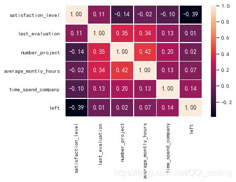
汇总以上结果，如下。

结论： 工作年限越长，月平均工作时长越长，最近一次评估结果越好，参与项目数量越多，员工越倾向于离职；员工满意度越低，员工越倾向于离职。
故，为了减少离职人数，降低离职率，采取措施如下

• 应将月平均工作时长调整在(155,235]之间；
• 最近一次评估结果靠近中
• 参与项目数超过2个，小于6个。参与项目书超过5个，离职率明显上升
• 提高员工工作年限，过了第五年，员工离职率明显下降，7年以后，离职率几乎为0
• 增加员工满意度，通过加薪/调查问卷/访谈等方式调研员工需求，并作出相应调整

2. 最低留存率工作年限员工离职的驱动力分析

做流失驱动力分析：即在流失率最高的年份，寻找当年员工流失的主要因素是什么？

# 保留一份原始数据
data_df2 = df.copy()

time_left_1 = data_df2[data_df2.left==1].groupby('time_spend_company')['left'].count()
time_all = data_df2.groupby('time_spend_company')['left'].count()
# 分别计算离职人数和在职人数所占比例
time_left_1_rate = time_left_1/time_all
time_left_1_rate = time_left_1_rate.fillna(0)
time_left_0_rate = 1-time_left_1_rate
y1 = [round(i,2) for i in time_left_1_rate.values.reshape(8,).tolist()]
y2 = [round(i,2) for i in time_left_0_rate.values.reshape(8,).tolist()]

c = (
    Bar()
    .add_xaxis(time_all.index.tolist())
    .add_yaxis('离职', y1, stack="stack1")
    .add_yaxis('在职', y2, stack="stack1")
    .set_series_opts(label_opts=opts.LabelOpts(is_show=False))
    .set_global_opts(title_opts=opts.TitleOpts(title="工作年限与是否离职的关系图"))
)
c.render_notebook()

结论: 流失率最高的工作年限为5年的员工。

我们筛选工作年限>=5的员工；新建一个特征来表示是否在第五年流失

注意： 比较第n年离职与否的人时候，第n年没离职的人的特征可能会受到他在第x年之后工作情况的影响，但我们假设这种影响是微弱的，所以我们认为在数据中 这两类人群所对应的特征还是有可比性的。

提取工作年限大于等于5年的数据

# 从模型ready的数据框data_df2中筛选5年及以上的人员数据
year5_df = data_df2[data_df2['time_spend_company']>=5]
# 增加一列平均项目用时
year5_df['平均项目用时'] =  year5_df['average_montly_hours']*year5_df['time_spend_company']*12 / year5_df['number_project']
# 增加一列年均项目数
year5_df['年均项目数'] = year5_df['number_project'] / year5_df['time_spend_company']
# 增加一列“第五年离职”
year5_df['第五年离职'] = np.where((year5_df['time_spend_company']==5) & (year5_df['left']==1), 1, 0)
# year5_df.head()

分类变量预处理

我们发现所有特征中，职务序列和薪资水平不是数值类型。需要将两个特征转换成对模型友好的全数值类型。(因为要训练模型，所有要用将分类特征转化为数字特征的数据框）

# 将薪资水平转化成整数型(转成1,2,3)
map_ = {
     'low':1, 'medium':2,'high':3}
year5_df['salary']= year5_df['salary'].map(map_)
year5_df.head()

## 自定义一个“独热编码”方程
## 将一个数据框（df）中的所有分类特征（cols）转换成哑变量特征
def one_hot(df, cols):
    for each in cols:
        dummies = pd.get_dummies(df[each], prefix=each, drop_first=False)
        dummies = dummies.drop(dummies.columns[len(dummies.columns)-1], axis=1) ## 每一组哑变量会自动删除最后一列（作为参考值）
        df = pd.concat([df, dummies], axis=1)
    df.drop(cols, axis = 1, inplace = True)
    return df
## 使用定义好的“独热编码”方程度当前的训练、测试集进行变换
year5_df = one_hot(year5_df, ["sales"])
year5_df.head()

	satisfaction_level	last_evaluation	number_project	average_montly_hours	time_spend_company	Work_accident	left	promotion_last_5years	salary	平均项目用时	...	第五年离职	sales_IT	sales_RandD	sales_accounting	sales_hr	sales_management	sales_marketing	sales_product_mng	sales_sales	sales_support
1	0.80	0.86	5	262	6	0	1	0	2	3772.8	...	0	0	0	0	0	0	0	0	1	0
3	0.72	0.87	5	223	5	0	1	0	1	2676.0	...	1	0	0	0	0	0	0	0	1	0
7	0.92	0.85	5	259	5	0	1	0	1	3108.0	...	1	0	0	0	0	0	0	0	1	0
8	0.89	1.00	5	224	5	0	1	0	1	2688.0	...	1	0	0	0	0	0	0	0	1	0
12	0.84	0.92	4	234	5	0	1	0	1	3510.0	...	1	0	0	0	0	0	0	0	1	0

5 rows × 21 columns

# 切分数据
X = year5_df.drop(['第五年离职'],axis = 1)
y = year5_df['第五年离职']

2.1 决策树

建模分析 - 基于决策树对最低留存率年限的驱动力分析

from sklearn.tree import DecisionTreeClassifier
from sklearn import tree
from IPython.display import Image  
import graphviz 
import pydotplus
import os
os.environ["PATH"] += os.pathsep + 'C:/Program Files (x86)/Graphviz2.38/bin'

DTclf = DecisionTreeClassifier(max_depth=5, min_samples_leaf=100,class_weight = 'balanced')
DTclf.fit(X, y)
# 决策树可视化笔记：
## 参考：https://blog.csdn.net/llh_1178/article/details/78516774
## 1. 需要单独从官网上下载Graphviz（for windows: http://www.graphviz.org/Download_windows.php）
## 2. 下载相关库：pip install graphviz
## 3. 在代码中导入graphviz的路径（os.environ["PATH"] += os.pathsep + 'C:/Program Files (x86)/Graphviz2.38/bin'）
## 4. 具体画图代码参考：https://scikit-learn.org/stable/modules/tree.html
dot_data = tree.export_graphviz(DTclf, out_file=None,
                         # 对应特征的名字       
                         feature_names=X.columns.values,   
                         filled=True, rounded=True,  
                         special_characters=True)
graph = graphviz.Source(dot_data)
graph 

2.2 逻辑回归

import numpy as np
import pandas as pd
from patsy import dmatrices
from sklearn.linear_model import LogisticRegression
from sklearn.model_selection import train_test_split
from sklearn import metrics
import matplotlib.pyplot as plt
import seaborn as sns
import warnings
from sklearn.preprocessing import StandardScaler
import statsmodels.api as sm
from statsmodels.stats.outliers_influence import variance_inflation_factor
plt.rcParams["font.family"] = "SimHei"
plt.rcParams["axes.unicode_minus"] = False 
plt.rcParams["font.size"] = 12 
warnings.filterwarnings("ignore")

vif_calc_df = year5_df.drop([ '第五年离职', 'left'], axis=1)

# 计算当前所有特征的VIF值
vif = pd.DataFrame()
vif["Features"] = vif_calc_df.columns
vif["VIF Factor"] = [variance_inflation_factor(vif_calc_df.values, i) for i in range(vif_calc_df.shape[1])]
pd.set_option('display.max_rows',None)
vif

	Features	VIF Factor
0	satisfaction_level	6.969022
1	last_evaluation	25.694318
2	number_project	321.573079
3	average_montly_hours	77.777796
4	time_spend_company	127.366280
5	Work_accident	1.213808
6	promotion_last_5years	1.157826
7	salary	8.349769
8	平均项目用时	55.158268
9	年均项目数	154.975388
10	sales_IT	1.481379
11	sales_RandD	1.290273
12	sales_accounting	1.293144
13	sales_hr	1.265811
14	sales_management	1.685760
15	sales_marketing	1.369685
16	sales_product_mng	1.360867
17	sales_sales	2.758246
18	sales_support	1.821956

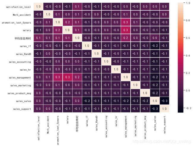
# 相关系数矩阵热力图
f,ax = plt.subplots(figsize=(12, 8))
sns.heatmap(vif_calc_df.corr(),annot=True,linewidths=.5,fmt= '.1f' ,ax = ax)
plt.show()

[外链图片转存失败,源站可能有防盗链机制,建议将图片保存下来直接上传(img-nPSPwNyi-1592816515655)(output_104_0.png)]

# 去除ID和预测量特征
vif_calc_df2 = year5_df.drop(['第五年离职','left','number_project','年均项目数','time_spend_company','last_evaluation'
                             ,'average_montly_hours'], axis=1)

# 计算当前所有特征的VIF值
vif = pd.DataFrame()
vif["Features"] = vif_calc_df2.columns
vif["VIF Factor"] = [variance_inflation_factor(vif_calc_df2.values, i) for i in range(vif_calc_df2.shape[1])]
vif

	Features	VIF Factor
0	satisfaction_level	4.818915
1	Work_accident	1.179708
2	promotion_last_5years	1.142846
3	salary	5.716008
4	平均项目用时	5.567143
5	sales_IT	1.349174
6	sales_RandD	1.190348
7	sales_accounting	1.228606
8	sales_hr	1.190463
9	sales_management	1.626398
10	sales_marketing	1.288461
11	sales_product_mng	1.271692
12	sales_sales	2.359087
13	sales_support	1.576902

# 相关性系数矩阵热力图
f,ax = plt.subplots(figsize=(12, 8))
sns.heatmap(data=vif_calc_df2.corr(),annot=True,linewidths=.5,fmt= '.1f',ax=ax)
plt.show()

选择最优自变量组合
使用逻辑回归模型，对各个特征的预测能力排序。

# 首先切分自变量和因变量
X = year5_df.drop(['第五年离职','number_project','年均项目数','time_spend_company','last_evaluation'
                             ,'average_montly_hours','left'], axis=1) # 排除引起多重共线性的特征
y = year5_df['第五年离职']

# 将数据标准化
from sklearn.preprocessing import StandardScaler
X_standard = StandardScaler().fit_transform(X)
X_standard = pd.DataFrame(data=X_standard, columns=list(X.columns)) 
# 呈现
X_standard.head()

	satisfaction_level	Work_accident	promotion_last_5years	salary	平均项目用时	sales_IT	sales_RandD	sales_accounting	sales_hr	sales_management	sales_marketing	sales_product_mng	sales_sales	sales_support
0	0.675774	-0.410924	-0.19001	0.591096	-0.046809	-0.29532	-0.225221	-0.222539	-0.215256	-0.268299	-0.251587	-0.253214	1.55776	-0.397555
1	0.380380	-0.410924	-0.19001	-0.970236	-0.661587	-0.29532	-0.225221	-0.222539	-0.215256	-0.268299	-0.251587	-0.253214	1.55776	-0.397555
2	1.118864	-0.410924	-0.19001	-0.970236	-0.419442	-0.29532	-0.225221	-0.222539	-0.215256	-0.268299	-0.251587	-0.253214	1.55776	-0.397555
3	1.008092	-0.410924	-0.19001	-0.970236	-0.654861	-0.29532	-0.225221	-0.222539	-0.215256	-0.268299	-0.251587	-0.253214	1.55776	-0.397555
4	0.823470	-0.410924	-0.19001	-0.970236	-0.194113	-0.29532	-0.225221	-0.222539	-0.215256	-0.268299	-0.251587	-0.253214	1.55776	-0.397555

from mlxtend.feature_selection import SequentialFeatureSelector
from mlxtend.feature_selection import SequentialFeatureSelector as SFS
from sklearn import linear_model
model = linear_model.LogisticRegression()
# 实例化SFS
sfs1 = SFS(model, 
           k_features=14, 
           forward=True, 
           #verbose=2, ## 运行时显示细节
           scoring='f1', ## 使用MAE作为评判依据
           cv=5, ## 5-fold 交叉验证
           n_jobs=-1) ## -1 表示使用当前所有的CPU去运行程序 
# 导入数据并运行
sfs1 = sfs1.fit(X_standard, y)

# 表格呈现特征选取的排名结果
pd.DataFrame.from_dict(sfs1.get_metric_dict()).T

## 可视化结果
from mlxtend.plotting import plot_sequential_feature_selection as plot_sfs
from matplotlib.pyplot import figure
plot_sfs(sfs1.get_metric_dict(), kind='std_err')
plt.title('Sequential Forward Selection (w. StdErr)')
# plt.ylim(0.82, 0.845)
plt.show()

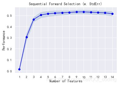
# 选取特定特征
feature_df = pd.DataFrame.from_dict(sfs1.get_metric_dict()).T
selected_features = list(feature_df.iloc[8]["feature_names"])
# 呈现
selected_features

['satisfaction_level',
 'Work_accident',
 'promotion_last_5years',
 'salary',
 '平均项目用时',
 'sales_hr',
 'sales_management',
 'sales_product_mng',
 'sales_sales']

在排除了导致多重共线性的特征后，我们进一步选择了最优自变量组合。我们将使用这些特征在下一步训练逻辑回归模型

lm = LogisticRegression()
lm.fit(X_standard[selected_features], y)

LogisticRegression()

# 输出拟合后的系数和相应的名称构成数据框
pd_df = pd.DataFrame(lm.coef_[0], index = X_standard[selected_features].columns,columns=['Coefficients'])
tmp_df = pd_df.sort_values(by='Coefficients', ascending=False)

# 驱动力排序
tmp_df['正向驱动/负向'] = np.where(tmp_df['Coefficients']>0,'+','-')
tmp_df['Coefficients'] = abs(tmp_df['Coefficients'])
tmp_df = tmp_df.sort_values(by = 'Coefficients',ascending =False)
tmp_df

	Coefficients	正向驱动/负向
平均项目用时	0.924421	-
satisfaction_level	0.705542	+
Work_accident	0.546058	-
promotion_last_5years	0.503605	-
salary	0.326210	-
sales_management	0.214019	-
sales_sales	0.068194	-
sales_product_mng	0.063897	-
sales_hr	0.014727	-

结论：
基于上一步的分析，我们发现在所有输入到模型的9个变量中，对在第五年离职与否的主要驱动力为：

• 平均项目用时长（项目复杂/重要/员工做的慢）的员工倾向于留职
• 员工满意度高，会使得员工在第五年离职（值得深入研究）
• 有工作事故的员工倾向于留职
• 近5年获得提升的员工倾向于留职
• 薪水越高的员工，越倾向于留职

这9个变量（分析第五年是否离职的维度）是我们在上面两步（去除多重共线性，选择最优自变量组合）中筛选出来的。在这个工程中，也需要考虑到业务同事的意见（比如他们认为保留哪些特征非常必要）。