Andrew NG 机器学习 练习5-Regularized Linear Regression and Bias/Variance

1 Regularized Linear Regression

本文根据水库中蓄水标线(water level) 使用正则化的线性回归模型预测 水流量(water flowing out of dam)，然后 debug 学习算法 以及 讨论偏差和方差对 该线性回归模型的影响。

1.1 Visualizing the dataset

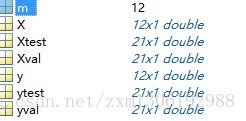
本作业的数据集分成三部分：
ⓐ训练集(training set)，样本矩阵(训练集)：X，结果标签(label of result)向量 y
ⓑ交叉验证集(cross validation set)，Xval 和 yval
ⓒ测试集(test set) ，Xtest 和 ytest

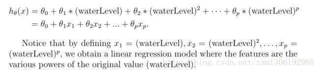
将数据加载到Matlab中如下：训练集中一共有12个训练实例，每个训练实例只有一个特征。故假设函数 hθ(x)=θ0⋅x0+θ1⋅x1 ，用向量表示成： hθ(x)=θT⋅x
一般地， x0 为 bais unit，默认 x0 ==1

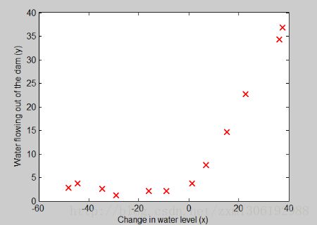
训练数据集中的数据图形表示如下：

%% =========== Part 1: Loading and Visualizing Data =============
%  We start the exercise by first loading and visualizing the dataset. 
%  The following code will load the dataset into your environment and plot
%  the data.
%

% Load Training Data
fprintf('Loading and Visualizing Data ...\n')

% Load from ex5data1: 
% You will have X, y, Xval, yval, Xtest, ytest in your environment
load ('ex5data1.mat');

% m = Number of examples
m = size(X, 1);

% Plot training data
plot(X, y, 'rx', 'MarkerSize', 10, 'LineWidth', 1.5);
xlabel('Change in water level (x)');
ylabel('Water flowing out of the dam (y)');

fprintf('Program paused. Press enter to continue.\n');
pause;

1.2 正则化线性回归模型的代价函数

线性回归的代价函数公式如下：

%% =========== Part 2: Regularized Linear Regression Cost =============
%  You should now implement the cost function for regularized linear 
%  regression. 
%

theta = [1 ; 1];
J = linearRegCostFunction([ones(m, 1) X], y, theta, 1);

fprintf(['Cost at theta = [1 ; 1]: %f '...
         '\n(this value should be about 303.993192)\n'], J);

fprintf('Program paused. Press enter to continue.\n');
pause;

linearRegCostFunction.m

function [J, grad] = linearRegCostFunction(X, y, theta, lambda)
%LINEARREGCOSTFUNCTION Compute cost and gradient for regularized linear 
%regression with multiple variables
%   [J, grad] = LINEARREGCOSTFUNCTION(X, y, theta, lambda) computes the 
%   cost of using theta as the parameter for linear regression to fit the 
%   data points in X and y. Returns the cost in J and the gradient in grad

% Initialize some useful values
m = length(y); % number of training examples

% You need to return the following variables correctly 
J = 0;
grad = zeros(size(theta));

% ====================== YOUR CODE HERE ======================
% Instructions: Compute the cost and gradient of regularized linear 
%               regression for a particular choice of theta.
%
%               You should set J to the cost and grad to the gradient.
%
reg = (lambda / (2*m)) * ( ( theta( 2:length(theta) ) )' * theta(2:length(theta)) );
J = sum((X*theta-y).^2)/(2*m) + reg;
% =========================================================================
grad = grad(:);

end

注意：由于θ0不参与正则化项的，故上面Matlab数组下标是从2开始的(Matlab数组下标是从1开始的，θ0是Matlab数组中的第一个元素)。

1.3 正则化的线性回归梯度

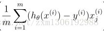
梯度的计算公式如下：

下面公式的向量表示就是： [XT⋅(X⋅θ−y)]/m ，用Matlab表示就是：X’*(X*theta-y) / m

梯度的Matlab代码实现如下：

grad_tmp = X'*(X*theta-y) / m;
grad = [ grad_tmp(1:1); grad_tmp(2:end) + (lambda/m)*theta(2:end) ];

1.4 拟合线性回归

%% =========== Part 4: Train Linear Regression =============
%  Once you have implemented the cost and gradient correctly, the
%  trainLinearReg function will use your cost function to train 
%  regularized linear regression.
% 
%  Write Up Note: The data is non-linear, so this will not give a great 
%                 fit.
%

%  Train linear regression with lambda = 0
lambda = 0;
[theta] = trainLinearReg([ones(m, 1) X], y, lambda);

%  Plot fit over the data
plot(X, y, 'rx', 'MarkerSize', 10, 'LineWidth', 1.5);
xlabel('Change in water level (x)');
ylabel('Water flowing out of the dam (y)');
hold on;
plot(X, [ones(m, 1) X]*theta, '--', 'LineWidth', 2)
hold off;

fprintf('Program paused. Press enter to continue.\n');
pause;

trainLinearReg.m

function [theta] = trainLinearReg(X, y, lambda)
%TRAINLINEARREG Trains linear regression given a dataset (X, y) and a
%regularization parameter lambda
%   [theta] = TRAINLINEARREG (X, y, lambda) trains linear regression using
%   the dataset (X, y) and regularization parameter lambda. Returns the
%   trained parameters theta.
%

% Initialize Theta
initial_theta = zeros(size(X, 2), 1); 

% Create "short hand" for the cost function to be minimized
costFunction = @(t) linearRegCostFunction(X, y, t, lambda);

% Now, costFunction is a function that takes in only one argument
options = optimset('MaxIter', 200, 'GradObj', 'on');

% Minimize using fmincg
theta = fmincg(costFunction, initial_theta, options);

end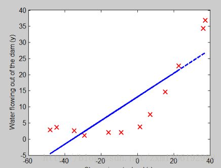

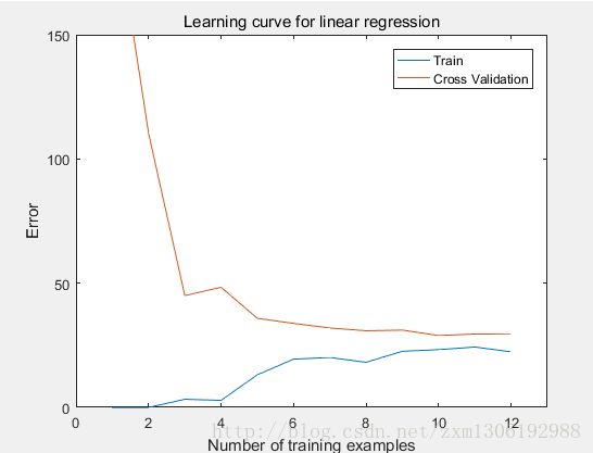
从上图中可以看出，由于我们的数据是二维的，但是却用一个线性模型去拟合，故很明显出现了 underfiting problem

在这里，我们很容易将模型以图形化方式表现出来，因为，我们的训练数据的特征很少(一维)。当训练数据的特征很多(feature variables)时，就很难画图了(三维以上很难直接用图形表示了…)。这时，就需要用 “学习曲线”来检查 训练出来的模型与数据是否很好地拟合了。

2 偏差与方差之间的权衡

高偏差—欠拟合，underfit
高方差—过拟合，overfit

可以用学习曲线(learning curve)来诊断 偏差–方差 问题。
学习曲线的 x 轴是训练集大小(training set size)，y 轴则是交叉验证误差和训练误差。

训练误差的定义如下：

注意：训练误差 Jtrain(θ) 不用正则化，因此在调用linearRegCostFunction时，lambda==0。

%% =========== Part 5: Learning Curve for Linear Regression =============
%  Next, you should implement the learningCurve function. 
%
%  Write Up Note: Since the model is underfitting the data, we expect to
%                 see a graph with "high bias" -- Figure 3 in ex5.pdf 
%

lambda = 0;
[error_train, error_val] = ...
    learningCurve([ones(m, 1) X], y, ...
                  [ones(size(Xval, 1), 1) Xval], yval, ...
                  lambda);

plot(1:m, error_train, 1:m, error_val);
title('Learning curve for linear regression')
legend('Train', 'Cross Validation')
xlabel('Number of training examples')
ylabel('Error')
axis([0 13 0 150])

fprintf('# Training Examples\tTrain Error\tCross Validation Error\n');
for i = 1:m
    fprintf('  \t%d\t\t%f\t%f\n', i, error_train(i), error_val(i));
end

fprintf('Program paused. Press enter to continue.\n');
pause;

Matlab实现如下(learningCurve.m)

function [error_train, error_val] = ...
    learningCurve(X, y, Xval, yval, lambda)
%LEARNINGCURVE Generates the train and cross validation set errors needed 
%to plot a learning curve
%   [error_train, error_val] = ...
%       LEARNINGCURVE(X, y, Xval, yval, lambda) returns the train and
%       cross validation set errors for a learning curve. In particular, 
%       it returns two vectors of the same length - error_train and 
%       error_val. Then, error_train(i) contains the training error for
%       i examples (and similarly for error_val(i)).
%
%   In this function, you will compute the train and test errors for
%   dataset sizes from 1 up to m. In practice, when working with larger
%   datasets, you might want to do this in larger intervals.
%

% Number of training examples
m = size(X, 1);

% You need to return these values correctly
error_train = zeros(m, 1);
error_val   = zeros(m, 1);

% ====================== YOUR CODE HERE ======================
% Instructions: Fill in this function to return training errors in 
%               error_train and the cross validation errors in error_val. 
%               i.e., error_train(i) and 
%               error_val(i) should give you the errors
%               obtained after training on i examples.
%
% Note: You should evaluate the training error on the first i training
%       examples (i.e., X(1:i, :) and y(1:i)).
%
%       For the cross-validation error, you should instead evaluate on
%       the _entire_ cross validation set (Xval and yval).
%
% Note: If you are using your cost function (linearRegCostFunction)
%       to compute the training and cross validation error, you should 
%       call the function with the lambda argument set to 0. 
%       Do note that you will still need to use lambda when running
%       the training to obtain the theta parameters.
%
% Hint: You can loop over the examples with the following:
%
%       for i = 1:m
%           % Compute train/cross validation errors using training examples 
%           % X(1:i, :) and y(1:i), storing the result in 
%           % error_train(i) and error_val(i)
%           ....
%           
%       end
%

% ---------------------- Sample Solution ----------------------

for i = 1:m
        theta = trainLinearReg(X(1:i, :), y(1:i), lambda);
        error_train(i) = linearRegCostFunction(X(1:i, :), y(1:i), theta, 0);
        error_val(i) = linearRegCostFunction(Xval, yval, theta, 0);

% -------------------------------------------------------------
% =========================================================================

end

学习曲线的图形如下：可以看出欠拟合时，在 training examples 数目很少时，训练出来的模型还能拟合”一点点数据”，故训练误差相对较小；但对于交叉验证误差而言，它是使用未知的数据得算出来到的，而现在模型欠拟合，故几乎不能 拟合未知的数据，因此交叉验证误差非常大。

随着 training examples 数目的增多，由于欠拟合，训练出来的模型越来越能拟合一些数据了，故训练误差增大了。而对于交叉验证误差而言，最终慢慢地与训练误差一致并变得越来越平坦，此时，再增加训练样本(training examples)已经对模型的训练效果没有太大影响了—在欠拟合情况下，再增加训练集的个数也不能再降低训练误差了。

3 多项式回归

从上面的学习曲线图形可以看出：出现了underfit problem，通过添加更多的特征(features)，使用更高幂次的多项式来作为假设函数拟合数据，以解决欠拟合问题。

多项式回归模型的假设函数如下：

%% =========== Part 6: Feature Mapping for Polynomial Regression =============
%  One solution to this is to use polynomial regression. You should now
% 

p = 8;

% Map X onto Polynomial Features and Normalize
X_poly = polyFeatures(X, p);
[X_poly, mu, sigma] = featureNormalize(X_poly);  % Normalize
X_poly = [ones(m, 1), X_poly];                   % Add Ones

% Map X_poly_test and normalize (using mu and sigma)
X_poly_test = polyFeatures(Xtest, p);
X_poly_test = bsxfun(@minus, X_poly_test, mu);
X_poly_test = bsxfun(@rdivide, X_poly_test, sigma);
X_poly_test = [ones(size(X_poly_test, 1), 1), X_poly_test];         % Add Ones

% Map X_poly_val and normalize (using mu and sigma)
X_poly_val = polyFeatures(Xval, p);
X_poly_val = bsxfun(@minus, X_poly_val, mu);
X_poly_val = bsxfun(@rdivide, X_poly_val, sigma);
X_poly_val = [ones(size(X_poly_val, 1), 1), X_poly_val];           % Add Ones

fprintf('Normalized Training Example 1:\n');
fprintf('  %f  \n', X_poly(1, :));

fprintf('\nProgram paused. Press enter to continue.\n');
pause; complete polyFeatures to map each example into its powers
%

通过对特征“扩充”，以添加更多的features，代码实现如下：polyFeatures.m

function [X_poly] = polyFeatures(X, p)
%POLYFEATURES Maps X (1D vector) into the p-th power
%   [X_poly] = POLYFEATURES(X, p) takes a data matrix X (size m x 1) and
%   maps each example into its polynomial features where
%   X_poly(i, :) = [X(i) X(i).^2 X(i).^3 ...  X(i).^p];
%


% You need to return the following variables correctly.
X_poly = zeros(numel(X), p);

% ====================== YOUR CODE HERE ======================
% Instructions: Given a vector X, return a matrix X_poly where the p-th 
%               column of X contains the values of X to the p-th power.
%
% 
for i = 1:p
    X_poly(:,i) = X.^i;
end
% =========================================================================

end

“扩充”了特征之后，就变成了多项式回归了，但由于多项式回归的特征取值范围差距太大（比如有些特征的取值很小，而有些特征的取值非常大），故需要用到Normalization(归一化)，归一化的代码如下：

featureNormalize.m

function [X_norm, mu, sigma] = featureNormalize(X)
%FEATURENORMALIZE Normalizes the features in X 
%   FEATURENORMALIZE(X) returns a normalized version of X where
%   the mean value of each feature is 0 and the standard deviation
%   is 1. This is often a good preprocessing step to do when
%   working with learning algorithms.

mu = mean(X);
X_norm = bsxfun(@minus, X, mu);

sigma = std(X_norm);
X_norm = bsxfun(@rdivide, X_norm, sigma);
% ============================================================
end

3.1 学习多项式回归

%% =========== Part 7: Learning Curve for Polynomial Regression =============
%  Now, you will get to experiment with polynomial regression with multiple
%  values of lambda. The code below runs polynomial regression with 
%  lambda = 0. You should try running the code with different values of
%  lambda to see how the fit and learning curve change.
%

lambda = 0;
[theta] = trainLinearReg(X_poly, y, lambda);

% Plot training data and fit
figure(1);
plot(X, y, 'rx', 'MarkerSize', 10, 'LineWidth', 1.5);
plotFit(min(X), max(X), mu, sigma, theta, p);
xlabel('Change in water level (x)');
ylabel('Water flowing out of the dam (y)');
title (sprintf('Polynomial Regression Fit (lambda = %f)', lambda));

figure(2);
[error_train, error_val] = ...
    learningCurve(X_poly, y, X_poly_val, yval, lambda);
plot(1:m, error_train, 1:m, error_val);

title(sprintf('Polynomial Regression Learning Curve (lambda = %f)', lambda));
xlabel('Number of training examples')
ylabel('Error')
axis([0 13 0 100])
legend('Train', 'Cross Validation')

fprintf('Polynomial Regression (lambda = %f)\n\n', lambda);
fprintf('# Training Examples\tTrain Error\tCross Validation Error\n');
for i = 1:m
    fprintf('  \t%d\t\t%f\t%f\n', i, error_train(i), error_val(i));
end

fprintf('Program paused. Press enter to continue.\n');
pause;

继续再用原来的linearRegCostFunction.m计算多项式回归的代价函数和梯度，得到的多项式回归模型的假设函数的图形如下：（注意：lambda==0，没有使用正则化）：

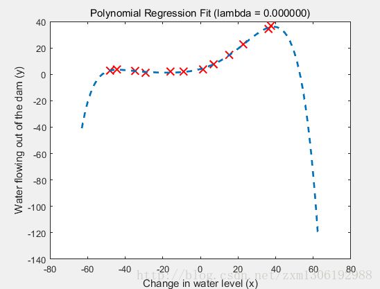
从多项式回归模型的 图形看出：它几乎很好地拟合了所有的训练样本数据。因此，可认为出现了：过拟合问题(overfit problem)—高方差

多项式回归模型的学习曲线 图形如下：

1. 

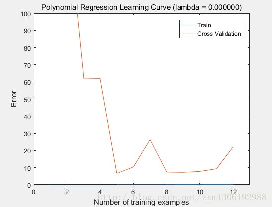
从多项式回归的学习曲线图形看出：训练误差几乎为0(非常贴近 x 轴了)，这正是因为过拟合—模型几乎完美地穿过了训练数据集中的每个数据点，从而训练误差非常小。

交叉验证误差先是很大(训练样本数目为2时)，然后随着训练样本数目的增多，cross validation error 变得越来越小了(训练样本数目2 增加到 5 过程中)；然后，当训练样本数目再增多时（11个以上的训练样本时…），交叉验证误差又变得大了(过拟合导致泛化能力下降)。

3.2 使用正则化来解决多项化回归模型的过拟合问题

设置正则化项 lambda =1(λ=1)时，得到的模型假设函数图形如下：

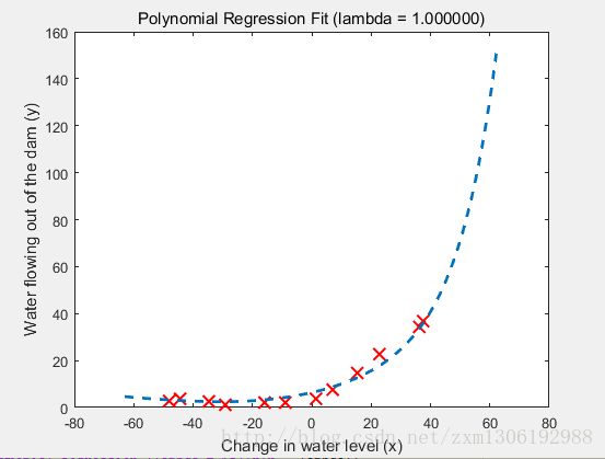
可以看出：这里的拟合曲线不再是 lambda = 0 时 那样弯弯曲曲的了，也不是非常精准地穿过每一个点，而是变得相对比较平滑。这正是 正则化 的效果。

lambda=1 (λ=1) 时的学习曲线如下：

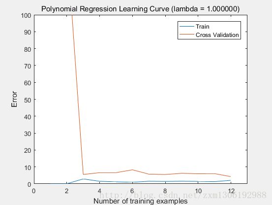
lambda==1时的学习曲线表明：该模型有较好的泛化能力，能够对未知的数据进行较好的预测。因为，它的交叉验证误差和训练误差非常接近，且非常小。（训练误差小，表明模型能很好地拟合数据，但有可能出现过拟合的问题，过拟合时，是不能很好地对未知数据进行预测的；而此处交叉验证误差也小，表明模型也能够很好地对未知数据进行预测）

最后来看下，多项式回归模型的正则化参数 lambda == 100(λ==100)时的情况：（出现了underfit problem–欠拟合–高偏差）

模型“假设函数”曲线如下：

学习曲线图形如下：

3.3 如何自动选择合适的 正则化参数 lambda(λ) ？

从第⑧点中看出：正则化参数 lambda(λ) 等于0时，出现了过拟合， lambda(λ) 等于100时，又出现了欠拟合， lambda(λ) 等于1时，模型刚刚好。

那在训练过程中如何自动选择合适的lambda参数呢？

可以使用交叉验证集(根据交叉验证误差来选择合适的 lambda 参数)

具体的选择方法如下：

首先有一系列的待选择的 lambda(λ) 值，在本λ作业中用一个lambda_vec向量保存这些 lambda 值（一共有10个）：

lambda_vec = [0 0.001 0.003 0.01 0.03 0.1 0.3 1 3 10]’

然后，使用训练数据集 针对这10个 lambda 分别训练 10个正则化的模型。然后对每个训练出来的模型，计算它的交叉验证误差，选择交叉验证误差最小的那个模型所对应的lambda(λ)值，作为最适合的 λ 。（注意：在计算训练误差和交叉验证误差时，是没有正则化项的，相当于 lambda=0）

for i = 1:length(lambda_vec)
   theta = trainLinearReg(X,y,lambda_vec(i));%对于每个lambda,训练出模型参数theta
   %compute jcv and jval without regularization,causse last arguments(lambda) is zero 
   error_train(i) = linearRegCostFunction(X, y, theta, 0);%计算训练误差
   error_val(i) = linearRegCostFunction(Xval, yval, theta, 0);%计算交叉验证误差
end

对于这10个不同的 lambda，计算出来的训练误差和交叉验证误差如下：

lambda      Train Error Validation Error
 0.000000   0.173616    22.066602
 0.001000   0.156653    18.597638
 0.003000   0.190298    19.981503
 0.010000   0.221975    16.969087
 0.030000   0.281852    12.829003
 0.100000   0.459318    7.587013
 0.300000   0.921760    4.636833
 1.000000   2.076188    4.260625
 3.000000   4.901351    3.822907
 10.000000  16.092213   9.945508

训练误差、交叉验证误差以及 lambda 之间的关系 图形表示如下：

当 lambda >= 3 的时候，交叉验证误差开始上升，如果再增大 lambda 就可能出现欠拟合了…

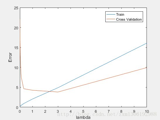
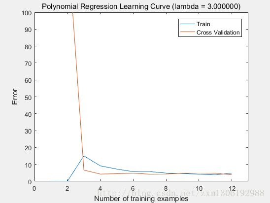
从上面看出：lambda == 3 时，交叉验证误差最小。lambda==3时的拟合曲线如下：（可与 lambda==1时的拟合曲线及学习曲线对比一下，看有啥不同）

学习曲线如下：

%% =========== Part 8: Validation for Selecting Lambda =============
%  You will now implement validationCurve to test various values of 
%  lambda on a validation set. You will then use this to select the
%  "best" lambda value.
%

[lambda_vec, error_train, error_val] = ...
    validationCurve(X_poly, y, X_poly_val, yval);

close all;
plot(lambda_vec, error_train, lambda_vec, error_val);
legend('Train', 'Cross Validation');
xlabel('lambda');
ylabel('Error');

fprintf('lambda\t\tTrain Error\tValidation Error\n');
for i = 1:length(lambda_vec)
    fprintf(' %f\t%f\t%f\n', ...
            lambda_vec(i), error_train(i), error_val(i));
end

fprintf('Program paused. Press enter to continue.\n');
pause;

validationCurve.m

function [lambda_vec, error_train, error_val] = ...
    validationCurve(X, y, Xval, yval)
%VALIDATIONCURVE Generate the train and validation errors needed to
%plot a validation curve that we can use to select lambda
%   [lambda_vec, error_train, error_val] = ...
%       VALIDATIONCURVE(X, y, Xval, yval) returns the train
%       and validation errors (in error_train, error_val)
%       for different values of lambda. You are given the training set (X,
%       y) and validation set (Xval, yval).
%

% Selected values of lambda (you should not change this)
lambda_vec = [0 0.001 0.003 0.01 0.03 0.1 0.3 1 3 10]';

% You need to return these variables correctly.
error_train = zeros(length(lambda_vec), 1);
error_val = zeros(length(lambda_vec), 1);

% ====================== YOUR CODE HERE ======================
% Instructions: Fill in this function to return training errors in 
%               error_train and the validation errors in error_val. The 
%               vector lambda_vec contains the different lambda parameters 
%               to use for each calculation of the errors, i.e, 
%               error_train(i), and error_val(i) should give 
%               you the errors obtained after training with 
%               lambda = lambda_vec(i)
%
% Note: You can loop over lambda_vec with the following:
%
%       for i = 1:length(lambda_vec)
%           lambda = lambda_vec(i);
%           % Compute train / val errors when training linear 
%           % regression with regularization parameter lambda
%           % You should store the result in error_train(i)
%           % and error_val(i)
%           ....
%           
%       end
%
%

for i = 1:length(lambda_vec)
   theta = trainLinearReg(X,y,lambda_vec(i));%对于每个lambda,训练出模型参数theta
   %compute jcv and jval without regularization,causse last arguments(lambda) is zero 
   error_train(i) = linearRegCostFunction(X, y, theta, 0);%计算训练误差
   error_val(i) = linearRegCostFunction(Xval, yval, theta, 0);%计算交叉验证误差
end
% =========================================================================

end

参考：http://www.cnblogs.com/hapjin/p/6114466.html