SSD模型物体检测（水下生物识别）

一，前期准备工作

1.下载SSD源码
下载地址，将checkpoints文件夹下的压缩包解压出来
2.在目录下新建三个文件夹：tfrecords_、train_model、VOC2007
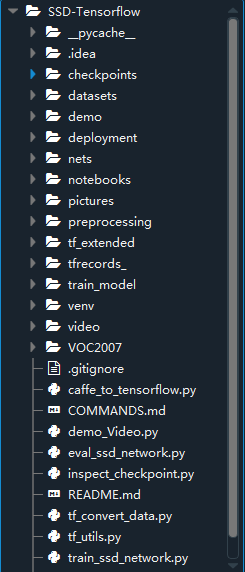
在spyder打开项目后结构如下：

二，数据集制作

1.采用VOC2007格式，使用labelImg，制作方法参考该文章:

这三个文件夹拖入到VOC2007文件夹中，JPEGImages存储图片，Annotations存储标签等信息.
2.将.xml标签，生成.tfrecord文件
在工程中新建一个py文件 transform.py，输入以下代码

# -*- coding：utf-8 -*-
# -*- author：zzZ_CMing  CSDN address:https://blog.csdn.net/zzZ_CMing
# -*- 2018/07/17; 13:18
# -*- python3.5
"""
特别注意: 17行VOC_LABELS标签要修改，189行的path地址要正确
"""

import os
import sys
import random
import numpy as np
import tensorflow as tf
import xml.etree.ElementTree as ET

# 我的标签定义只有手表这一类，所以下面的VOC_LABELS要根据自己的图片标签而定，第一组'none': (0, 'Background')是不能删除的；
VOC_LABELS = {
     
    'none': (0, 'Background'),
    'watch': (1, 'watch')
}

# 图片和标签存放的文件夹.
DIRECTORY_ANNOTATIONS = 'Annotations/'
DIRECTORY_IMAGES = 'JPEGImages/'

# 随机种子.
RANDOM_SEED = 4242
SAMPLES_PER_FILES = 3  # 每个.tfrecords文件包含几个.xml样本



def int64_feature(value):
    """
    生成整数型，浮点型和字符串型的属性
    """
    if not isinstance(value, list):
        value = [value]
    return tf.train.Feature(int64_list=tf.train.Int64List(value=value))


def float_feature(value):
    if not isinstance(value, list):
        value = [value]
    return tf.train.Feature(float_list=tf.train.FloatList(value=value))


def bytes_feature(value):
    if not isinstance(value, list):
        value = [value]
    return tf.train.Feature(bytes_list=tf.train.BytesList(value=value))


def _process_image(directory, name):
    """
    图片处理
    """
    # Read the image file.
    filename = directory + DIRECTORY_IMAGES + name + '.jpg'
    image_data = tf.gfile.FastGFile(filename, 'rb').read()

    # Read the XML annotation file.
    filename = os.path.join(directory, DIRECTORY_ANNOTATIONS, name + '.xml')
    tree = ET.parse(filename)
    root = tree.getroot()

    # Image shape.
    size = root.find('size')
    shape = [int(size.find('height').text),
             int(size.find('width').text),
             int(size.find('depth').text)]
    # Find annotations.
    bboxes = []
    labels = []
    labels_text = []
    difficult = []
    truncated = []
    for obj in root.findall('object'):
        label = obj.find('name').text
        labels.append(int(VOC_LABELS[label][0]))
        labels_text.append(label.encode('ascii'))  # 变为ascii格式

        if obj.find('difficult'):
            difficult.append(int(obj.find('difficult').text))
        else:
            difficult.append(0)
        if obj.find('truncated'):
            truncated.append(int(obj.find('truncated').text))
        else:
            truncated.append(0)

        bbox = obj.find('bndbox')
        a = float(bbox.find('ymin').text) / shape[0]
        b = float(bbox.find('xmin').text) / shape[1]
        a1 = float(bbox.find('ymax').text) / shape[0]
        b1 = float(bbox.find('xmax').text) / shape[1]
        a_e = a1 - a
        b_e = b1 - b
        if abs(a_e) < 1 and abs(b_e) < 1:
            bboxes.append((a, b, a1, b1))

    return image_data, shape, bboxes, labels, labels_text, difficult, truncated


def _convert_to_example(image_data, labels, labels_text, bboxes, shape,difficult, truncated):
    """
    转化样例
    """
    xmin = []
    ymin = []
    xmax = []
    ymax = []

    for b in bboxes:
        assert len(b) == 4
        # pylint: disable=expression-not-assigned
        [l.append(point) for l, point in zip([ymin, xmin, ymax, xmax], b)]
        # pylint: enable=expression-not-assigned

    image_format = b'JPEG'
    example = tf.train.Example(features=tf.train.Features(feature={
     
        'image/height': int64_feature(shape[0]),
        'image/width': int64_feature(shape[1]),
        'image/channels': int64_feature(shape[2]),
        'image/shape': int64_feature(shape),
        'image/object/bbox/xmin': float_feature(xmin),
        'image/object/bbox/xmax': float_feature(xmax),
        'image/object/bbox/ymin': float_feature(ymin),
        'image/object/bbox/ymax': float_feature(ymax),
        'image/object/bbox/label': int64_feature(labels),
        'image/object/bbox/label_text': bytes_feature(labels_text),
        'image/object/bbox/difficult': int64_feature(difficult),
        'image/object/bbox/truncated': int64_feature(truncated),
        'image/format': bytes_feature(image_format),
        'image/encoded': bytes_feature(image_data)}))
    return example


def _add_to_tfrecord(dataset_dir, name, tfrecord_writer):
    """
    增加到tfrecord
    """
    image_data, shape, bboxes, labels, labels_text, difficult, truncated = \
        _process_image(dataset_dir, name)
    example = _convert_to_example(image_data, labels, labels_text,
                                  bboxes, shape, difficult, truncated)
    tfrecord_writer.write(example.SerializeToString())


def _get_output_filename(output_dir, name, idx):
    """
    name为转化文件的前缀
    """
    return '%s/%s_%03d.tfrecord' % (output_dir, name, idx)


def run(dataset_dir, output_dir, name='voc_train', shuffling=False):
    if not tf.gfile.Exists(dataset_dir):
        tf.gfile.MakeDirs(dataset_dir)

    path = os.path.join(dataset_dir, DIRECTORY_ANNOTATIONS)
    filenames = sorted(os.listdir(path))
    if shuffling:
        random.seed(RANDOM_SEED)
        random.shuffle(filenames)

    i = 0
    fidx = 0
    while i < len(filenames):
        # Open new TFRecord file.
        tf_filename = _get_output_filename(output_dir, name, fidx)
        with tf.python_io.TFRecordWriter(tf_filename) as tfrecord_writer:
            j = 0
            while i < len(filenames) and j < SAMPLES_PER_FILES:
                sys.stdout.write(' Converting image %d/%d \n' % (i + 1, len(filenames)))  # 终端打印，类似print
                sys.stdout.flush()  # 缓冲

                filename = filenames[i]
                img_name = filename[:-4]
                _add_to_tfrecord(dataset_dir, img_name, tfrecord_writer)
                i += 1
                j += 1
            fidx += 1

    print('\nFinished converting the Pascal VOC dataset!')


def main(_):
    # 原数据集路径，输出路径以及输出文件名，要根据自己实际做改动
    dataset_dir = "../VOC2007_test/"
    output_dir = "tfrecords_/"
    if not os.path.exists(output_dir):
        os.mkdir(output_dir)

    run(dataset_dir, output_dir)


if __name__ == '__main__':
    tf.app.run()

运行后，文件将自动保存到tfrecords_文件夹

三、SSD框架细节调整

1.修改训练数据shape——打开datasets文件夹中的pascalvoc_2007.py文件，根据自己训练数据修改：NUM_CLASSES = 类别数；

2.修改类别个数——打开nets文件夹中的ssd_vgg_300.py文件，根据自己训练类别数修改96 和97行：等于类别数+1；
3.修改类别个数——打开eval_ssd_network.py文件，修改66行的类别个数：等于类别数+1；
4.修改训练步数epoch——打开train_ssd_network.py文件，
修改27行的数据格式，改为’NHWC’；
修改135行的类别个数：等于类别数+1；
修改154行训练总步数，None会无限训练下去；
5.下载vgg_16模型——下载地址请点击，密码：ge3x；下载完成解压后存入checkpoint文件中
四、训练模型
在SSD-Tensorflow文件夹中打开中断（shift+右键选择在终端中打开）
复制输入下面代码：

python ./train_ssd_network.py --train_dir=./train_model/
–dataset_dir=./tfrecords_/ --dataset_name=pascalvoc_2007 --dataset_split_name=train --model_name=ssd_300_vgg --checkpoint_path=./checkpoints/vgg_16.ckpt --checkpoint_model_scope=vgg_16 --checkpoint_exclude_scopes=ssd_300_vgg/conv6,ssd_300_vgg/conv7,ssd_300_vgg/block8,ssd_300_vgg/block9,ssd_300_vgg/block10,ssd_300_vgg/block11,ssd_300_vgg/block4_box,ssd_300_vgg/block7_box,ssd_300_vgg/block8_box,ssd_300_vgg/block9_box,ssd_300_vgg/block10_box,ssd_300_vgg/block11_box
–trainable_scopes=ssd_300_vgg/conv6,ssd_300_vgg/conv7,ssd_300_vgg/block8,ssd_300_vgg/block9,ssd_300_vgg/block10,ssd_300_vgg/block11,ssd_300_vgg/block4_box,ssd_300_vgg/block7_box,ssd_300_vgg/block8_box,ssd_300_vgg/block9_box,ssd_300_vgg/block10_box,ssd_300_vgg/block11_box
–save_summaries_secs=60 --save_interval_secs=600 --weight_decay=0.0005 --optimizer=adam --learning_rate=0.001 --learning_rate_decay_factor=0.94 --batch_size=24 --gpu_memory_fraction=0.9

–save_interval_secs是训练多少次保存参数的步长；
–optimizer是优化器；
–learning_rate是学习率；
–learning_rate_decay_factor是学习率衰减因子；
如果你的机器比较强大，可以适当增大–batch_size的数值，以及调高GPU的占比–gpu_memory_fraction
训练结束后进行测试
1、在日志中，选取最后一次生成模型作为测试模型进行测试，第48行；
2、在demo文件夹下放入测试图片；
3、最后在notebooks文件夹下建立demo_test.py测试文件，代码如下

# -*- coding：utf-8 -*-
# -*- author：zzZ_CMing  CSDN address:https://blog.csdn.net/zzZ_CMing
# -*- 2018/07/20; 15:19
# -*- python3.6
import os
import math
import random
import numpy as np
import tensorflow as tf
import cv2
import matplotlib.pyplot as plt
import matplotlib.image as mpimg
from nets import ssd_vgg_300, ssd_common, np_methods
from preprocessing import ssd_vgg_preprocessing
from notebooks import visualization
import sys

sys.path.append('../')
slim = tf.contrib.slim
# TensorFlow session: grow memory when needed. TF, DO NOT USE ALL MY GPU MEMORY!!!
gpu_options = tf.GPUOptions(allow_growth=True)
config = tf.ConfigProto(log_device_placement=False, gpu_options=gpu_options)
isess = tf.InteractiveSession(config=config)


# 定义数据格式，设置占位符
net_shape = (300, 300)
# 输入图像的通道排列形式，'NHWC'表示 [batch_size,height,width,channel]
data_format = 'NHWC'
# 预处理，以Tensorflow backend, 将输入图片大小改成 300x300，作为下一步输入
img_input = tf.placeholder(tf.uint8, shape=(None, None, 3))
# 数据预处理，将img_input输入的图像resize为300大小，labels_pre,bboxes_pre,bbox_img待解析
image_pre, labels_pre, bboxes_pre, bbox_img = ssd_vgg_preprocessing.preprocess_for_eval(
    img_input, None, None, net_shape, data_format, resize=ssd_vgg_preprocessing.Resize.WARP_RESIZE)
# 拓展为4维变量用于输入
image_4d = tf.expand_dims(image_pre, 0)

# 定义SSD模型
# 是否复用，目前我们没有在训练所以为None
reuse = True if 'ssd_net' in locals() else None
# 调出基于VGG神经网络的SSD模型对象，注意这是一个自定义类对象
ssd_net = ssd_vgg_300.SSDNet()
# 得到预测类和预测坐标的Tensor对象，这两个就是神经网络模型的计算流程
with slim.arg_scope(ssd_net.arg_scope(data_format=data_format)):
    predictions, localisations, _, _ = ssd_net.net(image_4d, is_training=False, reuse=reuse)

# 导入新训练的模型参数
ckpt_filename = '../train_model/model.ckpt-xxx'   # 注意xxx代表的数字是否和文件夹下的一致
# ckpt_filename = '../checkpoints/VGG_VOC0712_SSD_300x300_ft_iter_120000.ckpt'
isess.run(tf.global_variables_initializer())
saver = tf.train.Saver()
saver.restore(isess, ckpt_filename)

# 在网络模型结构中，提取搜索网格的位置
# 根据模型超参数，得到每个特征层（这里用了6个特征层，分别是4，7，8，9，10，11）的anchors_boxes
ssd_anchors = ssd_net.anchors(net_shape)
"""
每层的anchors_boxes包含4个arrayList，前两个List分别是该特征层下x，y坐标轴对于原图（300x300）大小的映射
第三,四个List为anchor_box的长度和宽度，同样是经过归一化映射的，根据每个特征层box数量的不同，这两个List元素
个数会变化。其中，长宽的值根据超参数anchor_sizes和anchor_ratios制定。
"""


# 主流程函数
def process_image(img, select_threshold=0.6, nms_threshold=.01, net_shape=(300, 300)):
    # select_threshold：box阈值——每个像素的box分类预测数据的得分会与box阈值比较，高于一个box阈值则认为这个box成功框到了一个对象
    # nms_threshold：重合度阈值——同一对象的两个框的重合度高于该阈值，则运行下面去重函数

    # 执行SSD模型，得到4维输入变量，分类预测，坐标预测，rbbox_img参数为最大检测范围，本文固定为[0,0,1,1]即全图
    rimg, rpredictions, rlocalisations, rbbox_img = isess.run([image_4d, predictions, localisations, bbox_img],
                                                              feed_dict={
     img_input: img})

    # ssd_bboxes_select()函数根据每个特征层的分类预测分数，归一化后的映射坐标，
    # ancohor_box的大小，通过设定一个阈值计算得到每个特征层检测到的对象以及其分类和坐标
    rclasses, rscores, rbboxes = np_methods.ssd_bboxes_select(
        rpredictions, rlocalisations, ssd_anchors,
        select_threshold=select_threshold, img_shape=net_shape, num_classes=21, decode=True)
    """
    这个函数做的事情比较多，这里说的细致一些：
    首先是输入，输入的数据为每个特征层（一共6个，见上文）的：
                                                rpredictions: 分类预测数据，
                                                rlocalisations: 坐标预测数据，
                                                ssd_anchors: anchors_box数据
                                            其中：
                                               分类预测数据为当前特征层中每个像素的每个box的分类预测
                                               坐标预测数据为当前特征层中每个像素的每个box的坐标预测
                                               anchors_box数据为当前特征层中每个像素的每个box的修正数据

        函数根据坐标预测数据和anchors_box数据，计算得到每个像素的每个box的中心和长宽，这个中心坐标和长宽会根据一个算法进行些许的修正，
    从而得到一个更加准确的box坐标；修正的算法会在后文中详细解释，如果只是为了理解算法流程也可以不必深究这个，因为这个修正算法属于经验算
    法，并没有太多逻辑可循。
        修正完box和中心后，函数会计算每个像素的每个box的分类预测数据的得分，当这个分数高于一个阈值（这里是0.5）则认为这个box成功
    框到了一个对象，然后将这个box的坐标数据，所属分类和分类得分导出，从而得到：
        rclasses：所属分类
        rscores：分类得分
        rbboxes：坐标
        
        最后要注意的是，同一个目标可能会在不同的特征层都被检测到，并且他们的box坐标会有些许不同，这里并没有去掉重复的目标，而是在下文
    中专门用了一个函数来去重
    """

    # 检测有没有超出检测边缘
    rbboxes = np_methods.bboxes_clip(rbbox_img, rbboxes)
    rclasses, rscores, rbboxes = np_methods.bboxes_sort(rclasses, rscores, rbboxes, top_k=400)
    # 去重，将重复检测到的目标去掉
    rclasses, rscores, rbboxes = np_methods.bboxes_nms(rclasses, rscores, rbboxes, nms_threshold=nms_threshold)
    # 将box的坐标重新映射到原图上（上文所有的坐标都进行了归一化，所以要逆操作一次）
    rbboxes = np_methods.bboxes_resize(rbbox_img, rbboxes)
    return rclasses, rscores, rbboxes


# 测试的文件夹
path = '../demo/z.jpg'
img = mpimg.imread(path)
rclasses, rscores, rbboxes = process_image(img)

# visualization.bboxes_draw_on_img(img, rclasses, rscores, rbboxes, visualization.colors_plasma)
visualization.plt_bboxes(img, rclasses, rscores, rbboxes)

结果演示：

参考