sql 线性回归_SQL Server中的Microsoft线性回归

sql 线性回归

In this article, we will be discussing Microsoft Linear Regression in SQL Server. This is the next data mining topic in our SQL Server Data mining techniques series. Naïve Bayes, Decision Trees, Time Series, Association Rules, and Clustering are the other techniques that we discussed until today.

在本文中，我们将讨论SQL Server中的Microsoft线性回归。 这是我们SQL Server数据挖掘技术系列中的下一个数据挖掘主题。 到目前为止，朴素贝叶斯，决策树，时间序列，关联规则和聚类是我们讨论的其他技术。

Microsoft Linear Regression is a forecasting technique. In this type of technique, there are multiple independent variables from which the dependent variable is predicted. For example, if you want to predict the house prices, you need to know the number of rooms, the area of the house, and other features of the house.

Microsoft线性回归是一种预测技术。 在这种技术中，存在多个自变量，从中可以预测因变量。 例如，如果要预测房价，则需要知道房间数量，房屋面积以及房屋的其他特征。

This means that the linear regression model can be represented as follows:

这意味着线性回归模型可以表示如下：

Let us see how we can use linear regression in the Microsoft SQL Server platform. As in the previous examples, today also, we will be using the vTargetMail view in the AdventureWorksDW sample database.

让我们看看如何在Microsoft SQL Server平台中使用线性回归。 和前面的示例一样，今天，我们还将在AdventureWorksDW示例数据库中使用vTargetMail视图。

As we did for other data mining techniques, first, we need to create a data source and the Data Source View. The Data source is chosen as AdventureWorksDW and vTargetMail view is selected as the data source views.

正如我们对其他数据挖掘技术所做的一样，首先，我们需要创建一个数据源和数据源视图。 选择数据源作为AdventureWorksDW，并选择vTargetMail视图作为数据源视图。

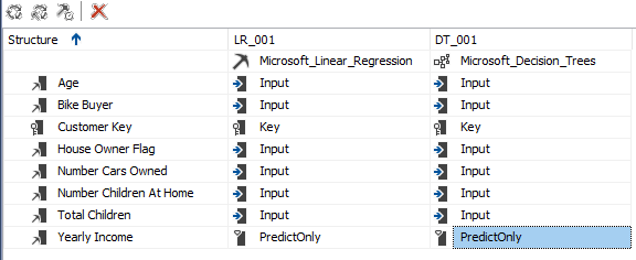
We choose the Microsoft Linear Regression as the data mining technique, as shown in the below screenshot.

我们选择Microsoft线性回归作为数据挖掘技术，如下面的屏幕快照所示。

In this technique, the Microsoft decision trees algorithm is used. Unlike in the decision trees, linear regression will have only one node, and we will verify the results for linear regression with the decision trees at the end of the article.

在此技术中，使用了Microsoft决策树算法。 与决策树不同，线性回归将只有一个节点，我们将在本文结尾处使用决策树验证线性回归的结果。

The vTargetMail will be the Case table and let us choose relevant attributes, as shown in the below screenshot.

vTargetMail将成为Case表，让我们选择相关属性，如下面的屏幕快照所示。

The Customer Key is chosen as the Key from the algorithm from the above screen. In Microsoft Linear regression, all the inputs should be numerical; the text column should not be selected. Therefore, in the above selection, Age, BikeBuyer, HouseOwnerFlag, NumberCarsOwned, NumberChildrenatHome, TotalChildren are selected as input attributes. This is a major limitation in the Microsoft Linear Regression, which is not in the standard Linear Regression techniques.

从以上屏幕的算法中，将客户密钥选择为密钥。 在Microsoft线性回归中，所有输入都应为数字； 不应选择文本列。 因此，在上述选择中，选择了Age，BikeBuyer，HouseOwnerFlag，NumberCarsOwned，NumberChildrenatHome，TotalChildren作为输入属性。 这是Microsoft线性回归中的主要限制，而标准线性回归技术中则没有。

In the previous examples, we have selected Bike Buyer as the predicted column. However, in the Microsoft Linear Regression, we are to predict YearlyIncome.

在前面的示例中，我们选择了“自行车购买者”作为预测列。 但是，在Microsoft线性回归中，我们将预测YearlyIncome。

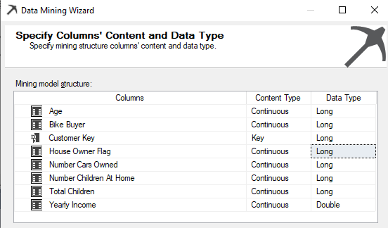
Though there are default Content types, there are instances where you need to change the content types. Content types can be modified from the following screenshot.

尽管存在默认的内容类型，但是在某些情况下您需要更改内容类型。 可以从以下屏幕截图中修改内容类型。

By default, House Owner Flag is selected Text data type, which has to be changed to the Long data type.

默认情况下，“ 房主标志”被选中为“文本”数据类型，必须将其更改为“长”数据类型。

In the other screens in the data mining wizard, default settings are used. This is the Solution Explorer for the Microsoft Linear Regression data mining technique.

在数据挖掘向导的其他屏幕中，使用默认设置。 这是Microsoft线性回归数据挖掘技术的解决方案资源管理器。

The next is to process the data mining structure. There will be a warning message saying that there is no split in decision trees. You can ignore this warning as for linear regression; there won’t be any split for the decision trees.

接下来是处理数据挖掘结构。 将出现一条警告消息，指出决策树中没有拆分。 对于线性回归，您可以忽略此警告。 决策树不会分裂。

After processing the data mining structure, we are now ready to view the results.

处理完数据挖掘结构后，我们现在可以查看结果了。

查看结果 (Viewing the Results)

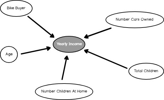
As we observed in many SQL Server algorithms, in linear regression, we can find the dependency network, as shown in the below screenshot.

正如我们在许多SQL Server算法中观察到的那样，在线性回归中，我们可以找到依赖关系网络，如下面的屏幕快照所示。

The Dependency network shows what the most dependent attributes to predict Yearly Income is. By sliding the slider down on the left-hand side, you can find out the significance of these attributes, as we observed in the Naïve base and Decision Trees.

依存关系网络显示了预测年收入的最依附属性。 通过在左侧向下滑动滑块，您可以找到这些属性的重要性，就像我们在朴素的基础和决策树中观察到的那样。

In Microsoft Linear Regression, only another available view is Tree View. However, as indicated before, it is a one-node tree view.

在Microsoft线性回归中，只有另一个可用的视图是“树视图”。 但是，如前所述，它是一个单节点树视图。

From this view, you can get the linear regression equation, which is the final goal of this technique.

从此视图中，您可以获得线性回归方程，这是该技术的最终目标。

The following screenshot shows the linear regression equation.

以下屏幕截图显示了线性回归方程。

This is the equation and you simply have to replace relevant values to predict the yearly income.

这就是方程式，您只需要替换相关值即可预测年收入。

Yearly Income = 57,308.498

年收入= 57,308.498

– 1,940.134*(Total Children-1.844)

– 1,940.134 *（儿童总数1.844）

+ 8,988.432*(Bike Buyer-0.494)

+ 8,988.432 *（自行车购买者-0.494）

+9,468.323*(Number Cars Owned-1.503)

+ 9,468.323 *（拥有汽车数量1.503）

+416.002*(Age-50.380)

+ 416.002 *（年龄50.380）

+7,818.527*(Number Children At Home-1.004)

+ 7,818.527 *（家庭儿童人数1.004）

Let us see how we can predict from the built model using prediction feature.

让我们看看如何使用预测功能从构建的模型进行预测。

预测 (Prediction)

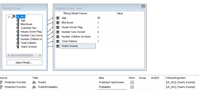
An important aspect of any data mining technique is to predict using the built model. Let us see how we can predict using the built Microsoft Linear Regression model. This can be done from the Mining Model Prediction tab, as shown in the below screenshot. In the following example, some values are provided for a given instance to predict the annual income.

任何数据挖掘技术的一个重要方面是使用构建的模型进行预测。 让我们看看如何使用内置的Microsoft线性回归模型进行预测。 可以从“挖掘模型预测”选项卡中完成，如下面的屏幕快照所示。 在以下示例中，为给定实例提供了一些值以预测年收入。

From the result tab, results can be views as shown in the below screenshot.

在结果选项卡中，结果可以是如下屏幕截图所示的视图。

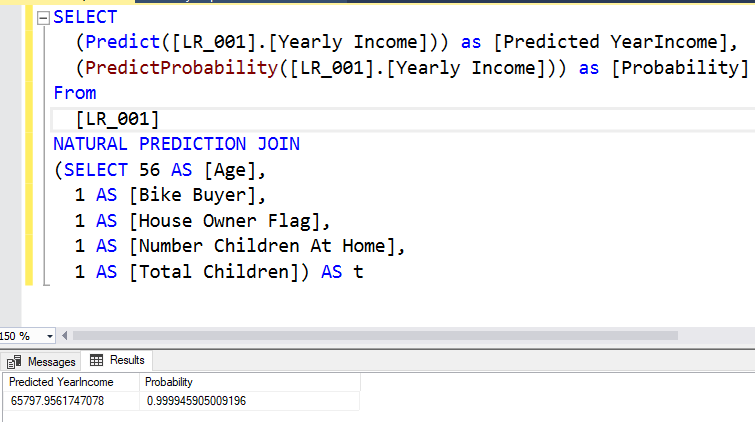
The same results can be obtained from SQL Server Management Studio by executing the DMX query. The following screenshot shows the query and its result.

通过执行DMX查询，可以从SQL Server Management Studio获得相同的结果。 以下屏幕截图显示了查询及其结果。

It is important to note that if you do not have some attributes, you can still obtain the results. The following screenshot shows the prediction value from the Linear Regression model when the number of cars is unknown.

重要的是要注意，如果没有某些属性，仍然可以获取结果。 以下屏幕截图显示了当汽车数量未知时来自线性回归模型的预测值。

When an attribute is missing, that attribute’s part will be ignored from the entire equation.

当缺少属性时，整个方程式将忽略该属性的一部分。

Let us validate the equation with the Decision Tree technique.

让我们用决策树技术验证方程。

决策树验证 (Validation with Decision Tree)

Adding another data mining technique in SQL Server is much simpler. You can add another mining model to the existing attributes in the Mining Model tab.

在SQL Server中添加另一种数据挖掘技术要简单得多。 您可以在“挖掘模型”选项卡中向现有属性添加另一个挖掘模型。

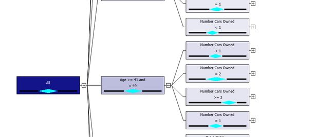
After processing the mining structure, you will observe the decision, as shown below.

处理完挖掘结构后，您将观察该决策，如下所示。

Let us look at the equation at the main node.

让我们看一下主节点上的等式。

Yearly Income = 57,308.215 + 9,468.574*(Number Cars Owned-1.503) + 415.816*(Age-50.384) + 8,988.666*(Bike Buyer-0.494) + 7,817.585*(Number Children At Home-1.004) – 1,939.209*(Total Children-1.844)

年收入= 57,308.215 + 9,468.574 *（拥有汽车数量1.503）+ 415.816 *（年龄50.384）+ 8,988.666 *（自行车购买者-0.494）+ 7,817.585 *（在家中儿童数量1.004）– 1,939.209 *（儿童总数1.844） ）

You will find that it is the same equation that you got from the linear regression.

您将发现它与线性回归得到的方程式相同。

More than that equation, the decision tree has the additional advantage of having node wise equation. In the decision trees, if you click every node, you find an equation, as shown in the below screenshot.

除了该方程式以外，决策树还具有节点式方程式的额外优势。 在决策树中，如果单击每个节点，则会找到一个方程式，如下面的屏幕快照所示。

This means that equation Yearly Income will be as 63,702.121-42,567.214*(House Owner Flag-0.733)+36,322.044*(Bike Buyer-0.500) is valid for Age >= 41 and < 49 and Number of cars owned = 2 and Total children = 1.

这意味着等式年收入将为63,702.121-42,567.214 *（房主旗帜-0.733）+ 36,322.044 *（自行车购买者-0.500）适用于年龄> = 41和<49以及拥有的汽车数量= 2和儿童总数= 1。

The following table shows the different equations at different nodes in the tree.

下表显示了树中不同节点上的不同方程式。

Data Set	Equation
Age >= 73 and < 81 and Total Children = 3	Yearly Income = 56,936.254-4,193.080*(Bike Buyer-0.121)-20,137.503*(Number Cars Owned-1.994)-1,936.065*(Age-75.146)
Total Children = 3 and Age = 76	Yearly Income = 58,000.000-8,884.447*(Bike Buyer-0.100)
Age = 73 and Total Children = 3	Yearly Income = 56,998.501+4,498.500*(Bike Buyer-0.333)
Age >= 73 and < 81 and Total Children = 2 and Number Children At Home = 3	Yearly Income = 121,037.417+2,108.061*(Age-75.667)+14,848.268*(Bike Buyer-0.333)
Age >= 49 and < 51 and Total Children >= 4 and Number Cars Owned = 2 and Number Children At Home < 3	Yearly Income = 62,583.618-18,114.343*(Number Children At Home-1.897)+5,525.516*(Bike Buyer-0.793)+6,861.981*(Age-49.759)-14,461.923*(Total Children-4.017)

数据集	方程
年龄> = 73且<81，儿童总数= 3	年收入= 56,936.254-4,193.080 *（自行车购买者-0.121）-20,137.503 *（拥有汽车数量1.994）-1,936.065 *（年龄75.146）
儿童总数= 3，年龄= 76	年收入= 58,000.000-8,884.447 *（自行车购买者-0.100）
年龄= 73，儿童总数= 3	年收入= 56,998.501 + 4,498.500 *（自行车购买者-0.333）
年龄> = 73并且<81，儿童总数= 2，家庭儿童数量= 3	年收入= 121,037.417 + 2,108.061 *（年龄75.667）+ 14,848.268 *（自行车购买者0.333）
年龄> = 49和<51，儿童总数> = 4，拥有的汽车数量= 2，家庭儿童数量<3	年收入= 62,583.618-18,114.343 *（在家中儿童的数量为1.897）+ 5,525.516 *（自行车购买者为-0.793）+ 6,861.981 *（年龄为49.759）-14,461.923 *（儿童总数为4.017）

This means that decision trees are more accurate than Microsoft linear regression.

这意味着决策树比Microsoft线性回归更准确。

型号参数 (Model Parameters)

As we discussed, every data mining technique has its parameters to suit your data and environments.

正如我们所讨论的，每种数据挖掘技术都有适合您的数据和环境的参数。

FORCE_REGRESSOR (FORCE_REGRESSOR)

Microsoft Linear Regression algorithm detects best-fitted attributes automatically and generates the linear equation. In this attempt, it might drop some attributes. However, you can force any attribute that you wish to include in the equation by including in the FORCE_REGRESSOR parameters. If there are multiple attributes, you can include all attributes, such as {Attribute 1}, {Attribute 2}.

Microsoft线性回归算法可自动检测最适合的属性并生成线性方程。 在这种尝试中，它可能会删除一些属性。 但是，可以通过包含在FORCE_REGRESSOR参数中来强制希望包含在公式中的任何属性。 如果有多个属性，则可以包括所有属性，例如{Attribute 1}，{Attribute 2}。

摘要 (Summary)

In this article, we discussed Linear regression as a forecasting technique. Microsoft Linear Regression technique was built on the Decision trees and we identified that the decision trees could be used as a regression technique as well.

在本文中，我们讨论了将线性回归作为一种预测技术。 Microsoft线性回归技术建立在决策树上，我们确定了决策树也可以用作回归技术。

目录 (Table of contents)

Introduction to SQL Server Data Mining

Naive Bayes Prediction in SQL Server

Microsoft Decision Trees in SQL Server

Microsoft Time Series in SQL Server

Association Rule Mining in SQL Server

Microsoft Clustering in SQL Server

Microsoft Linear Regression in SQL Server

Implement Artificial Neural Networks (ANNs) in SQL Server

Implementing Sequence Clustering in SQL Server

Measuring the Accuracy in Data Mining in SQL Server

Data Mining Query in SSIS

Text Mining in SQL Server

SQL Server数据挖掘简介

SQL Server中的朴素贝叶斯预测

SQL Server中的Microsoft决策树

SQL Server中的Microsoft时间序列

SQL Server中的关联规则挖掘

SQL Server中的Microsoft群集

SQL Server中的Microsoft线性回归

在SQL Server中实现人工神经网络（ANN）

在SQL Server中实现序列聚类

在SQL Server中测量数据挖掘的准确性

SSIS中的数据挖掘查询

SQL Server中的文本挖掘

翻译自: https://www.sqlshack.com/microsoft-linear-regression-in-sql-server/

sql 线性回归