吴恩达机器学习课程-作业1-线性回归（python实现）

Machine Learning(Andrew) ex1-Linear Regression

椰汁学习笔记

最近刚学习完吴恩达机器学习的课程，现在开始复习和整理一下课程笔记和作业，我将陆续更新。

---

Linear regression with one variable

• 2.1 Plotting the Data

首先我们读入数据，先观察数据的内容

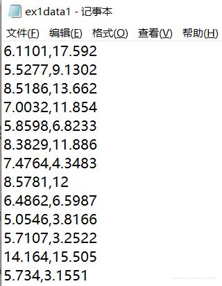
数据是一个txt文件，每一行存储一组数据，第一列数据为城市的人口，第二列数据城市饭店的利润。
读入数据时按行读入，每行通过分解，获得两个数据。数据的存储使用列表。初次接触没有使用一些第三方库pandas、numpy，后续会逐渐用到。

    # Part1：从txt文件中读取数据，绘制成散点图
    f = open("ex1data1.txt", 'r')
    population = []
    profit = []
    for line in f.readlines():
        col1 = line.split(',')[0]
        col2 = line.split(',')[1].split('\n')[0]
        population.append(float(col1))
        profit.append(float(col2))

接下来将数据可视化，需要用到matplotlib这个画图库，这个教程还可以

	import matplotlib.pyplot as plt
	#上面这样引入
    plt.title("Scatter plot of training data")
    plt.xlabel("population of city")
    plt.ylabel("profit")
    plt.scatter(population, profit, marker='x')
    plt.show()

xlabel和ylabel设置当前图片的x，y轴的标签；scatter绘制散点图，前两个参数为两个坐标轴的对应数值列表（元组等），marker指定绘制点的图形；show函数显示。

• 2.2 Gradient Descent

$$J(\theta )=\frac{1}{2m}\sum _{i=1}^m{h}_{\theta }(x^{(i)}-y^{(i)}{)}^2$$
$$h_{\theta }(x)={\theta }^{T}x={\theta }_0+{\theta }_1{x}_1$$

实现损失函数的计算

c = 0
theta = [0, 0] 
for j in range(m):
   c += 1.0 / (2 * m) * pow(theta[0] + theta[1] * population[j] - profit[j], 2)

当theta全部初始化为0时，结果为32.072733877455676

$${\theta }_j={\theta }_j-\alpha \frac{1}{m}\sum _{i=1}^m(h_{\theta }(x^{(i)}-y^{(i)}))x_j^{(i)}\text{(simultaneously update θj for all j)}$$
在这里第一次进行梯度下降编码，没有使用向量化的编码，只使用for循环遍历，求解。
在进行梯度下降编码时我们首先要弄清楚参数

    alpha = 0.01 #学习速率
    iterations = 1500 #梯度下降的迭代轮数
    theta = [0, 0] #初始化theta

接下来就是梯度下降实现了，第一个循环表示迭代轮数，第二个循环应该是遍历theta，这里数据的维数为二维，相应的theta也只有两个，因此省去了循环。 最内层循环遍历所有数据集。
注意课程中反复强调的所有参数同步更新，需要将计算的theta暂存，所有theta更新完毕后，同时修改原来的theta参数。

    # part2：递归下降，同时记录损失值的变化
    m = len(population)
    alpha = 0.01
    iterations = 1500
    theta = [0, 0]
    for i in range(iterations):
        temp0 = theta[0]
        temp1 = theta[1]
        for j in range(m):
            temp0 -= (alpha / m) * (theta[0] + theta[1] * population[j] - profit[j])
            temp1 -= (alpha / m) * (theta[0] + theta[1] * population[j] - profit[j]) * population[j]
        theta[0] = temp0
        theta[1] = temp1

• 2.3 Debugging

下面我们再绘制出最后拟合出来的直线，首先根据数据的范围随意确定X轴头尾两点，再使用拟合出的theta计算出对应的y值，再使用plot函数画出两点及连线。

    # part3：绘制回归直线图，已经损失函数变化图
    x = [5.0, 22.5]
    y = [5.0 * theta[1] + theta[0], 22.5 * theta[1] + theta[0]]
    plt.plot(x, y, color="red")
    plt.title("Linear Regression")
    plt.xlabel("population of city")
    plt.ylabel("profit")
    plt.scatter(population, profit, marker='x')

• 2.4 Visualizing J(θ)

为了判断拟合结果，可以将损失值随梯度下降过程的变化曲线绘出，帮助我们理解。这里没有像作业上绘制theta和cost的图像，只是简单的绘制cost的变化曲线。因为我觉得这个图理解效果一样。

    plt.title("Visualizing J(θ)")
    plt.xlabel("iterations")
    plt.ylabel("cost")
    plt.plot(t, cost, color="red")
    # t为迭代轮数，cost为每轮的损失值，这个计算要插入到梯度下降过程中，计算和记录。

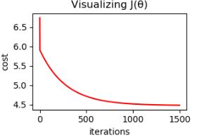
可以看到，损失值变化是一直下降，最后保持。因此我们的参数选择是比较好的。特别是学习速率不能取太大，会导致越来越偏离最优值。

---

Linear regression with multiple variables

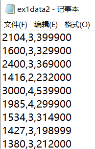
首先读入数据，此次的数据，特征包括第一列房子面积，第二列房间个数；第三列为价格。

    # 读入数据
    f = open("ex1data2.txt", 'r')
    house_size = []
    bedroom_number = []
    house_price = []
    for line in f.readlines():
        col1 = float(line.split(",")[0])
        col2 = float(line.split(",")[1])
        col3 = float(line.split(",")[2].split("\n")[0])
        house_size.append(col1)
        bedroom_number.append(col2)
        house_price.append(col3)

• 3.1 Feature Normalization

由于存在多个变量，需要将变量进行归一化，目的是使每个特征对结果影响不被数据数量级影响。
归一化的方法有很多，这篇博客有讲
这里我使用min-max标准化，将数据映射到[-1,1]
$$x_{normalized}=\frac{x-mean}{ptp},mean=average,ptp=max-min$$
从此开始我将使用numpy，教程在这，实现如下。由于y的数值也很大，我一并将其归一化。

    # 特征归一化
    x1 = np.array(house_size).reshape(-1, 1)
    x2 = np.array(bedroom_number).reshape(-1, 1)
    y = np.array(house_price).reshape(-1, 1)
    data = np.concatenate((x1, x2, y), axis=1)  # 放在一个ndarray中便于归一化处理

    mean = np.mean(data, axis=0)  # 计算每一列的均值
    ptp = np.ptp(data, axis=0)  # 计算每一列的最大最小差值
    nor_data = (data - mean) / ptp  # 归一化
    X = np.insert(nor_data[..., :2], 0, 1, axis=1)  # 添加x0=1
    y = nor_data[..., -1]

更常用的归一化方法是zero-mean normalization
$$x_{normalized}=\frac{x-\mu }{\sigma },\mu 为均值，\sigma 为方差$$
实现方法

    mean = np.mean(data, axis=0)
    std = np.std(data, axis=0, ddof=1) #除数为m-ddof，ddof默认为0
    nor_data = (data - mean) / std

不采用这个方法的原因是，会导致在使用正规矩阵求解是第一个参数为0，还不清楚其中的原因。

• 3.2 Gradient Descent

这里我们使用完全向量化的实现方法，ndarray.dot()为点乘即是内积，可以用@运算符代替，ndarray.T为当前转置。

def gradient_descent(X, theta, y, alpha, iterations):
    m = X.shape[0]
    c = []  # 存储计算损失值
    for i in range(iterations):
        theta -= (alpha / m) * X.T.dot(X.dot(theta) - y)
        c.append(cost(X, theta, y))
    return theta, c

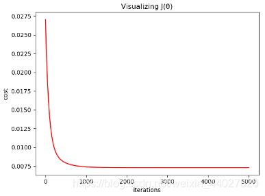
在这里每次梯度下降计算了当前的损失值，用于debug。画出损失值变化曲线。

    # 可视化下降过程
    plt.title("Visualizing J(θ)")
    plt.xlabel("iterations")
    plt.ylabel("cost")
    plt.plot([i for i in range(iterations)], c, color="red")
    plt.show()

当alpha=0.1,iterations=5000时曲线如下：
theta = [-2.47585640e-17 9.52353893e-01 -6.58737388e-02]

• 3.3 Normal Equations

正规方程可以一次计算出theta，根据矩阵变换：
$$\theta =(X^{T}X{)}^{-1}{X}^{T}y$$
使用numpy可以很方便的实现：

def normal_equation(X, y):
    return np.linalg.pinv(X.T.dot(X)).dot(X.T).dot(y)

推荐使用numpy.linalg.pinv()求矩阵的逆
这个方法求解theta只适用在数据量比较小的情况，因为矩阵求逆是个计算复杂度很高的操作。梯度下降的适用性更广。
对比发现，两种方法求出的theta会存在微小不同

---

完整的代码会同步在我的github

欢迎指正错误
学习的时候参考了Cowry，非常感谢。