python机器学习手写算法系列——DBSCAN聚类

本文，就像本系列的其他文章一样。旨在通过阅读原论文+手写代码的方式，自己先把算法搞明白，然后再教其他人。手写代码除了可以验证自己是否搞明白以外，我会对中间过程做图。这样，我可以通过图直观的验证算法是否正确。而这些图，又成为写文章时候的很好的素材。

什么是 DBSCAN

DBSCAN，全称是 Density-Based Scan。 故名思意，就是通过密度扫描。DBSCAN是一种聚类算法，和KMeans相比，他不需要指定cluster的数量。他的主要参数有两个，半径和邻居的数量。Scikit-Learn中，半径用$ϵ$(epsilon)表示，邻居的数量用min-samples表示。我们这里也借用sklearn的表示方式。这样大家使用sklearn的时候不会搞混。

当然，除了sklearn，在weka，R，elki等库里，也有DBSCAN的实现。他在教科书里也经常被提及，并有很多成功的实际运用。许多基于密度的聚类算法，也都受了DBSCAN的启发。实践证明改算法是有效的，并在2014年获得了SIGKDD的test-of-time大奖。

和KMeans比较

为什么有了KMeans，还要有DBSCAN，肯定是KMeans有解决不了的问题。

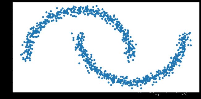
比如，我们画两个月亮。

import numpy as np
from matplotlib import pyplot as plt
from matplotlib.patches import Circle
from sklearn.cluster import DBSCAN, KMeans
from sklearn.datasets import make_moons
from sklearn.metrics.pairwise import euclidean_distances

X, y = make_moons(n_samples=1000, noise=0.05, random_state=42)
plt.figure(figsize=(12, 6))
plt.scatter(X[:,0], X[:,1])
plt.show()

然后，我们用KMeans聚类：

km = KMeans(n_clusters=2)
km.fit(X)
plt.figure(figsize=(12, 6))
# Plot the clusters
plt.scatter(X[:, 0], X[:, 1], c=km.labels_)
plt.title(f"Kmeans (k=2)")
plt.show()

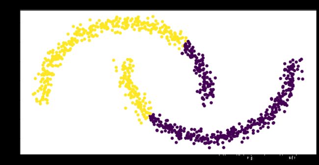
这里，我们可以看到，我们本来希望两个月亮能分别对应两个簇（cluster），但是事与愿违。这是因为，KMeans是按照距离来聚类的。一个月亮的边缘，距离其中心的距离，可能大于其距离另一个月亮中心的距离。这样，这些点就被另一个月亮带跑了。

DBSCAN 算法

第一步：找核心（core）点

这时，DBSCAN就出现了。他不是基于距离的，而是基于密度的。他把高密度的区域都连起来，形成一个簇。

这里，我们就需要半径（$ϵ$）和最小邻居数量（min-samples）来确定高密度区了。

首先，我们要找到一些中心点。他们的半径（$ϵ$）之内，有min-samples个点。我们这里把epsilon和min-samples设置为0.1和10。

这时找到的这些中心点，叫做core。

# set the parameters
epsilon = 0.1
min_samples = 10
# In most of the cluster algorithms, the first step is to calculate the distance matrix.
distance_matrix=euclidean_distances(X)
neighbour_predicate_matrix = distance_matrix<=epsilon
neighbour_counts_array=neighbour_predicate_matrix.sum(axis=0)
core_predicates = neighbour_counts_array>=min_samples
indices = np.arange(0, 1000)
core_indices = indices[core_predicates]
non_core_indices = indices[~core_predicates]
n_cores = sum(core_predicates)
n_non_cores = 1000-n_cores

plt.figure(figsize=(12, 6))
# cores
plt.scatter(X[core_indices,0], X[core_indices,1], c='r', label=f"cores({n_cores})" )
plt.scatter(X[non_core_indices,0], X[non_core_indices,1], c='g', label=f"non cores({n_non_cores})")
plt.legend()
plt.title("Cores and Non-cores")
plt.show()

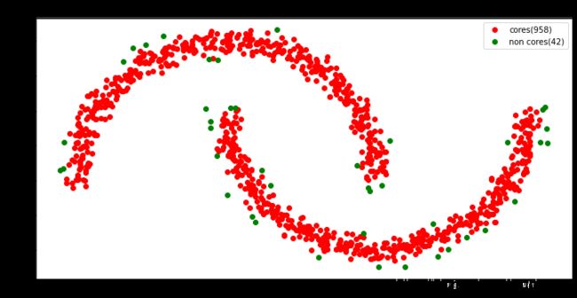
上图用红色表示core，用绿色表示non-core。

第二步：连接核心点

用了这些core，我们就要把他们都连接起来了。

labels = -np.ones((1000,), dtype=np.int)
cluster_id=0
loop_index=0
while sum(labels<0) > 0:
    #unlabelled_predicates = (labels==-1)
    unlabelled_core_predicates = ((core_predicates) & (labels==-1))
    unlabelled_core_indices = indices[unlabelled_core_predicates]
    if len(unlabelled_core_indices) == 0:
        break
    first_index=unlabelled_core_indices[0]
    neighbourhood_predicates = neighbour_predicate_matrix[first_index]
    neighbourhood_indices = indices[core_predicates & neighbourhood_predicates]
    
    while(len(neighbourhood_indices)>0):
        fig, ax = plt.subplots(figsize=(12, 6))
        fig.facecolor='white'
        circle = Circle((X[first_index, 0], X[first_index, 1]), 0.1, facecolor='none',
                        edgecolor=(0, 0.8, 0.8), linewidth=3, alpha=0.5)
        ax.add_patch(circle)

        # plt.figure(figsize=(10, 8))
        # cores
        plt.scatter(X[core_indices,0], X[core_indices,1], c='r')
        plt.scatter(X[non_core_indices,0], X[non_core_indices,1], c='g')
        # clustered
        plt.scatter(X[labels>=0,0], X[labels>=0,1], c=labels[labels>=0])
        # and its neighourhood
        plt.scatter(X[neighbourhood_indices, 0], X[neighbourhood_indices, 1], c="tab:blue", marker='o')
        # draw first 
        plt.scatter(X[first_index, 0], X[first_index, 1], c="tab:cyan", marker='o')
        plt.title(f"Cluster {cluster_id}, Loop {loop_index}")
        plt.show()
        # plt.savefig(f"tmp/{loop_index}.png")
        plt.clf()
        
        labels[neighbourhood_indices] = cluster_id
        unlabelled_predicates = (labels==-1)
        neighbourhood_predicates_matrix = neighbour_predicate_matrix[neighbourhood_indices]
        neighbourhood_predicates = neighbourhood_predicates_matrix.any(axis=0)
        
        neighbourhood_indices = indices[(core_predicates & neighbourhood_predicates & unlabelled_predicates)]
        
        loop_index+=1
        # break
    cluster_id+=1

我把这里打印的64张fig做成了gif。我们看到。算法先找到一个core，然后找到他半径($ϵ$)之内的core，把他们聚为一簇。然后，再找这个core的相邻的core，并置为一簇。以此类推，知道找不到新的core为止。这时，在剩下的core里，有发起一个新的簇。用上面的方法继续找，直到找不到为止。

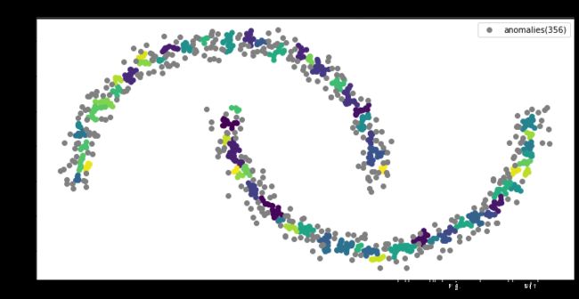
第三步：连接非核心点，并找出异常点

剩下的非核心点，我们可以直接认为都是异常点，也可以看他们是否在核心点的旁边，如果是，则继承核心点的簇，否则为异常点。这个完全看需要了。

clusters = np.unique(labels) 
for cluster_id in [c for c in clusters if c>-1]:
    # find the points that are already clusterd to cluster_id
    cluster_predicates = labels==cluster_id
    # find the neighours of the above
    neighbours_matrix = neighbour_predicate_matrix[cluster_predicates]
    neighbours_predicates = neighbours_matrix.any(axis=0)
    # remove the already clustered points from the neighourhood.
    clustered_non_core_indices=indices[neighbours_predicates & ~cluster_predicates]
    # label the rest neighours.
    labels[clustered_non_core_indices] = cluster_id

plt.figure(figsize=(12, 6))
# cores
#plt.scatter(X[core_indices,0], X[core_indices,1], c='r')
#plt.scatter(X[non_core_indices,0], X[non_core_indices,1], c='g')
anomaly_predicates = labels==-1
# clustered
plt.scatter(X[~anomaly_predicates,0], X[~anomaly_predicates,1], c=labels[labels>=0])
# anomalies

n_anomalies = sum(anomaly_predicates)
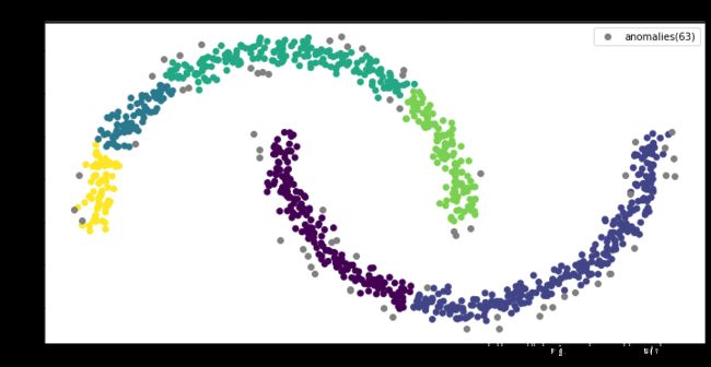
plt.scatter(X[anomaly_predicates,0], X[anomaly_predicates,1], c='gray', label=f'anomalies({n_anomalies})')
plt.legend()
plt.title("DBSCAN (from scratch) with epsilon=0.1 and min_samples=10")
plt.show()

最终，我们得到了两个分开的月亮，和三个异常点。

和scikit-learn比较

def cluster_and_plot(epsilon, min_samples):
    dbscan = DBSCAN(eps=epsilon, min_samples=min_samples)
    dbscan.fit(X)
    plt.figure(figsize=(12, 6))
    # Plot the clusters
    plt.scatter(X[dbscan.labels_>-1, 0], X[dbscan.labels_>-1, 1], c=dbscan.labels_[dbscan.labels_>-1])
    # plot anomolies
    anomaly_predicates = dbscan.labels_==-1
    n_anomalies = sum(anomaly_predicates)
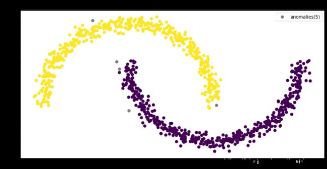
    plt.scatter(X[anomaly_predicates, 0], X[anomaly_predicates, 1], c='gray', label=f'anomalies({n_anomalies})')
    plt.title(f"SCAN with epsilon={epsilon} and min_samples={min_samples}")
    plt.legend()
    plt.show()
    
cluster_and_plot(0.1, 10)

我们看到，scikit-learn的结果和我们手写算法的结果是一致的。证明我们对算法的理解正确。

参数选择的启发

根据DBSCAN的作者们最新的论文，min-samples参数建议为2 * 维度。当效果不好的时候，可以增大。

$ϵ$比较难设置。根据算法的设计，$ϵ$越小越好。当然，这个也受距离算法的影响。专家经验也可以运用到$ϵ$的选择。比如在GPS地图上，$ϵ$设置为1公里。

这里，我们对上面的数据做了几个实验。我们保持min-samples=4（2*dim）不变，然后调整$ϵ$。我们看到当$ϵ$为0.03和0.04的时候，效果并不好。然后，我们增大$ϵ$到0.06，这时两个月亮被正确的分开了。接着，我们正大$ϵ$，我们看到异常点的数量在下降。

我想，在实际项目中，还是要根据实际情况区设置算法的参数的。比如，我们现在用DBSCAN去找信用卡行为异常。这时，银行可能要验证我们的算法，我们需要给银行一个最异常的客户。这时，我们就可以增大$ϵ$，以减少异常点。

但是如果反过来，另一个项目，预算也有效，他们只想找出最典型的客户，也是越少越好。这时别说异常点了，可能非核心点都要去掉。

总结

DBSCAN是一个神奇的算法，他即是聚类算法，又是异常检测算法。和KMeans不同，他把连续的区域聚为一类。我们应该根据实际需要选择算法及参数。当然，前提是你首先要了解这些算法。

代码地址

https://github.com/EricWebsmith/machine_learning_from_scrach

参考资料

书: Hands-on Machine Learning with Scikit-Learn and Tensorflow

论文: DBSCAN Revisited, Revisited: Why and How You Should (Still) Use DBSCAN