李宏毅机器学习2020HW1——手推线性回归公式预测PM2.5

前言

  这个是课程第一个作业，用线性回归模型做PM2.5的预测，优化方法用Adagrad，李老师提供了训练集和测试集以及示例代码，并推荐使用Linux或者Mac系统来做作业。而我准备用win10系统来完成这项作业。

一、要求

  给定训练集train.csv和测试集test.csv，要求根据前9个小时的空气监测情况预测第10个小时的PM2.5含量。

二、环境

  Win10系统，使用Pycharm，Python3.7。

三、数据介绍

  首先熟悉一下数据，训练集train.csv包含每个月前20天的完整观测数据，因为数据的编码方式是big5，使用Pycharm打开文件后显示乱码，先选择文件编码方式为“Big5-HKSCS”，reload之后就能正常打开。
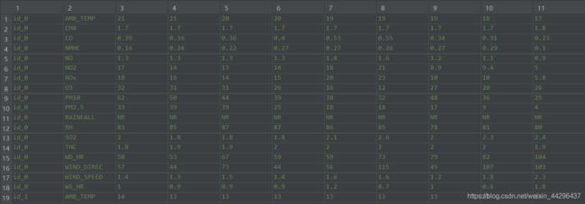
  训练集包含2014年1-12月中每个月前20天的数据，每个小时均记录一次数据，每次记录18个特征数据，包括AMB_TEMP, CH4, CO, NHMC, NO, NO2, NOx, O3, PM10, PM2.5, RAINFALL, RH, SO2, THC, WD_HR, WIND_DIREC, WIND_SPEED, WS_HR。其中RAINFALL指标的值不是数值格式。总共有4230行、24列有效数据（4320 = 12个月20天18个特征），部分训练集数据如下图。
  测试集test.csv的格式与训练集类似，共有240个id（类似训练集的240个日期），每个id有18项特征，均有9个小时的数据，以此来预测第10小时的PM2.5。总共有240行、9列有效数据。部分测试集数据如下图所示。

四、训练集数据预处理

  在Pycharm中新建一个Python工程，在venv文件夹中新建文件夹data，将train.csv和test.csv放入其中。

1. 数据清洗

  训练集中前三列不是数值部分，因此要从第四列开始取值，且需要将RAINFALL行的内容‘NR’替换为数值（以0代替）。

import pandas as pd
import numpy as np
data = pd.read_csv('./data/train.csv', encoding='Big5')
data = data.iloc[:, 3:] #iloc是根据行列号来取数据
data[data == 'NR'] = 0 #将RAINFALL行的字符替换为0
raw_data = data.to_numpy() #转换为numpy数组

  清洗完后，raw_data大小为4320*24。

2. 提取特征

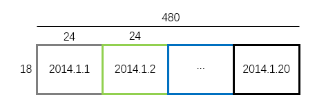
  按月份来看，清洗后的数据（raw_data）是可看成由12份360*24的二维数组组成（360 = 20天*18个特征）。将每份360*24的数组转换成18*480的数组，如下图所示。

  转换后的数组将变成如下形式：

  将12组18*480数组以放入一个字典中。

month_data = {
     } 
for month in range(12):
    sample = np.empty([18, 480]) #空的18*480数组
    for day in range(20):
        sample[:, day*24:(day+1)*24] = raw_data[18*(day+20*month):18*(day+1+20*month), :]
    month_data[month] = sample

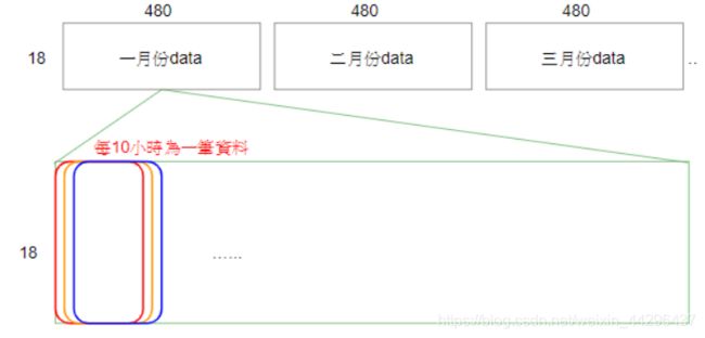
  由于最终目的是根据前9小时的数据预测第10小时的PM2.5，所以要把10小时的数据分为一组，其中前9小时的18*9个特征作为输入x，第10个小时的第10个特征作为输出y。上述转换后的18*480数组中，480列依次为同一个月1号到20号各小时的数据，也就是480个小时的数据。以1月份的数据为例，1-10列是1-10小时的数据，作为第1组数据；2-11列是2-10小时的数据，作为第2组数据；以步长为1的方式取值到第480列为止。如下图所示。

  这样，一个月就有471组数据，12个月就有12*471组数据，每组数据中，前9小时的数据（18*9的数组）转换成18*9维行向量作为输出；将第10小时的数据（18维列向量）中的第10行的数据（即第10个特征PM2.5的值）作为输出。12个月的12*471组数据的输出放入总的输入x中（12*471行，18*9列的数组），同理输出y为12*471维列向量。
  reshape(1, -1)：转换成一个行向量

x = np.empty([12*471, 18*9], dtype=float)
y = np.empty([12*471, 1], dtype=float)
for month in range(12):
    for day in range(20):
        for hour in range(24):
            if hour > 14 and day == 19:
                continue
            x[month*471 + day*24 + hour, :] = month_data[month][:, day*20 + hour:day*20 + hour + 9].reshape(1, -1)
            y[month*471 + day*24 + hour, :] = month_data[month][9, day*20 + hour + 9]

3. 标准化

  方法是减去列均值再除以列标准差。
  np.mean()：求均值。axis = 0：压缩行，对各列求均值，返回 1* n 矩阵。
  np.std()：求标准差。axis=0：计算每一列的标准差。

mean_x = np.mean(x, axis = 0) #18 * 9 
std_x = np.std(x, axis = 0) #18 * 9 
for i in range(len(x)): #12 * 471
    for j in range(len(x[0])): #18 * 9 
        if std_x[j] != 0:
            x[i][j] = (x[i][j] - mean_x[j]) / std_x[j]
#print(x)

六、训练

  模型：线性回归

$$\begin{gathered} \mathbf{y}=\left[\begin{array}{c}{y}_1\\ y_2\\ ⋮\\ y_m\end{array}\right]=\left[\begin{array}{c}b+w_1{x}_{1,1}+w_2{x}_{1,2}+...+w_n{x}_{1,n}\\ b+w_1{x}_{2,1}+w_2{x}_{2,2}+...+w_n{x}_{2,n}\\ ⋮\\ b+w_1{x}_{m,1}+w_2{x}_{m,2}+...+w_n{x}_{m,n}\end{array}\right] \\ =\left[\begin{array}{ccccc}1& x_{1,1}& x_{1,2}& \cdots & x_{1,n}\\ 1& x_{2,1}& x_{2,2}& \cdots & x_{2,n}\\ ⋮& ⋮& ⋮& \ddots & ⋮\\ 1& x_{m,1}& x_{m,2}& \cdots & x_{m,n}\end{array}\right]\left[\begin{array}{c}b\\ w_1\\ w_2\\ ⋮\\ w_n\end{array}\right]=\left[\begin{array}{c}{\mathbf{x}}_1\\ {\mathbf{x}}_2\\ ⋮\\ {\mathbf{x}}_m\end{array}\right]\mathbf{w}=\mathbf{X}\mathbf{w} \\ n=18\ast 9，m=12\ast 471 \end{gathered}$$
  损失函数：均方根误差
$$L(\mathbf{w})=\sqrt{\frac{1}{m}\sum _{i=1}^m(y_i-{\hat{y}}_i{)}^2}=\sqrt{\frac{1}{m}\sum _{i=1}^m({\mathbf{x}}_i\mathbf{w}-{\hat{y}}_i{)}^2}，m=12\ast 471$$
  优化方法：Adagrad
$${\mathbf{w}}^{t+1}={\mathbf{w}}^t-\frac{{\eta }^t}{{\sigma }^t}\frac{\partial L({\mathbf{w}}^t)}{\partial {\mathbf{w}}^t}$$
$${\sigma }^t=\sqrt{\frac{1}{t+1}\sum _{i=0}^t{\left(\frac{\partial L({\mathbf{w}}^i)}{\partial {\mathbf{w}}^i}\right)}^2}$$
$${\eta }^t=\frac{\eta }{\sqrt{t+1}}$$
  化简后可得Adagrad的优化公式：
$${\mathbf{w}}^{t+1}={\mathbf{w}}^t-\frac{\eta }{\sqrt{{\sum }_{i=0}^t{\left(\frac{\partial L({\mathbf{w}}^i)}{\partial {\mathbf{w}}^i}\right)}^2}}\frac{\partial L({\mathbf{w}}^t)}{\partial {\mathbf{w}}^t}$$
  为减少梯度$\frac{\partial L({\mathbf{w}}^t)}{\partial {\mathbf{w}}^t}$的计算量，将$L(\mathbf{w})$简化为$Loss={\sum }_{i=1}^m({\mathbf{x}}_i\mathbf{w}-{\hat{y}}_i{)}^2$来求梯度，其中，$({\mathbf{x}}_i\mathbf{w}-{\hat{y}}_i{)}^2=(b+x_{i,1}{w}_1+x_{i,2}{w}_2+\cdots +x_{i,n}{w}_n{)}^2$。即：$$\begin{gathered} \frac{\partial L({\mathbf{w}}^t)}{\partial {\mathbf{w}}^t}=\left[\begin{array}{c}\frac{\partial L({\mathbf{w}}^t)}{\partial b^t}\\ \frac{\partial L({\mathbf{w}}^t)}{\partial w_1^t}\\ ⋮\\ \frac{\partial L({\mathbf{w}}^t)}{\partial w_n^t}\end{array}\right]=2\left[\begin{array}{c}1({\mathbf{x}}_1\mathbf{w}-{\hat{y}}_1)+1({\mathbf{x}}_2\mathbf{w}-{\hat{y}}_2)+\cdots +1({\mathbf{x}}_m\mathbf{w}-{\hat{y}}_m)\\ x_{1,1}({\mathbf{x}}_1\mathbf{w}-{\hat{y}}_1)+x_{2,1}({\mathbf{x}}_2\mathbf{w}-{\hat{y}}_2)+\cdots +x_{m,1}({\mathbf{x}}_m\mathbf{w}-{\hat{y}}_m)\\ ⋮\\ x_{1,n}({\mathbf{x}}_1\mathbf{w}-{\hat{y}}_1)+x_{2,n}({\mathbf{x}}_2\mathbf{w}-{\hat{y}}_2)+\cdots +x_{m,n}({\mathbf{x}}_m\mathbf{w}-{\hat{y}}_m)\end{array}\right] \\ =2\left[\begin{array}{cccc}1& 1& \cdots & 1\\ x_{1,1}& x_{2,1}& \cdots & x_{m,1}\\ x_{1,2}& x_{2,2}& \cdots & x_{m,2}\\ ⋮& ⋮& \ddots & ⋮\\ x_{1,n}& x_{2,n}& \cdots & x_{m,n}\end{array}\right]\left(\left[\begin{array}{c}{\mathbf{x}}_1\mathbf{w}\\ {\mathbf{x}}_2\mathbf{w}\\ ⋮\\ {\mathbf{x}}_m\mathbf{w}\end{array}\right]-\left[\begin{array}{c}{\hat{y}}_1\\ {\hat{y}}_2\\ ⋮\\ {\hat{y}}_m\end{array}\right]\right)=2{\mathbf{X}}^T\left(\mathbf{X}\mathbf{w}-\hat{\mathbf{y}}\right) \end{gathered}$$
  np.zeros([m,n])：返回一个全0的m*n数组。
  np.ones([m,n])：返回一个全1的m*n维数组。
  np.concatenate((a,b),axis=1)：a和b做行拼接，结果为[a,b]。
  np.dot(x,w)：x和w点乘。
  np.power(x,n)：x中各元素的n次方。
  np.sqrt(x)：x中各元素的平方根。
  np.sum(x)：x中所有元素的和，返回一个值。
  x.transpose()：将x转置。

dim = 18 * 9 + 1 #参数：18*9个权重 + 1个偏置bias
w = np.zeros([dim, 1]) #参数列向量初始化为0
#x新增一列用来与偏置bias相乘，将模型y=wx+b转化成y=[b,w]转置·[1,x]
x = np.concatenate((np.ones([12 * 471, 1]), x), axis = 1).astype(float)
learning_rate = 1 
iter_time = 1000
adagrad = np.zeros([dim, 1])
eps = 0.0000000001
for t in range(iter_time):
    loss = np.sqrt(np.sum(np.power(np.dot(x, w) - y, 2))/471/12)#rmse
    if(t%100==0):
        print(str(t) + ":" + str(loss))
    gradient = 2 * np.dot(x.transpose(), np.dot(x, w) - y) #dim*1
    adagrad += gradient ** 2
    w = w - learning_rate * gradient / np.sqrt(adagrad + eps) #eps是一个很小的正数，避免分母为0
np.save('weight.npy', w)
#print(w)

七、测试

  测试集数据与训练集类似，不过只给了9个小时的数据，第10小时的数据需要用训练的模型预测。总共有240个id的数据，也就是240组18*9的数据，需要预测出240个值。

1. 数据预处理

  首先，测试集需要数据预处理，过程类似于对训练集做预处理。有一点需要注意，测试集的第一行就是数据，而pd.read_csv()在读取数据时，默认把第一行看作列号（非数据），因此在使用该函数时，要添加参数设置：header=None。

testdata = pd.read_csv('./data/test.csv', header=None, encoding='Big5')
test_data = testdata.iloc[:, 2:]
test_data[test_data == 'NR'] = 0
test_data = test_data.to_numpy()
test_x = np.empty([240, 18*9], dtype=float)
for i in range(240):
    test_x[i, :] = test_data[18*i: 18*(i + 1), :].reshape(1, -1)
std_test_x = np.std(test_x, axis=0)
mean_test_x = np.mean(test_x, axis=0)
for i in range(len(test_x)):
    for j in range(len(test_x[0])):
        if std_test_x[j] != 0:
            test_x[i][j] = (test_x[i][j] - mean_test_x[j]) / std_test_x[j]
test_x = np.concatenate((np.ones([240, 1]), test_x), axis = 1).astype(float)
#print(test_x)

2. 预测

  最后进行预测，将结果为负数的项替换为0。

w = np.load('weight.npy')
ans_y = np.dot(test_x, w)
for i in range(240):
    if(ans_y[i]<0):
        y[i] = 0
#print(ans_y)

  将结果保存到csv文件中。

import csv
with open('submit.csv', mode='w', newline='') as submit_file:
    csv_writer = csv.writer(submit_file)
    header = ['id', 'value']
    print(header)
    csv_writer.writerow(header)
    for i in range(240):
        row = ['id_' + str(i), ans_y[i][0]]
        csv_writer.writerow(row)
        print(row)