ML&DL - PyTorch系列学习笔记06——PyTorch进阶教程
ML&DL - PyTorch系列学习笔记06——PyTorch进阶教程
- 06 PyTorch进阶教程
-
- 6.1 Broadcasting
-
- Broadcasting操作的实际意义
- 实现Broadcasting操作的前提条件
- 6.2 Tensor拼接与拆分
-
- 拼接
- 切分
- 6.3 基本数学运算
-
- add+/minus-/multiply×/divide÷
- matmul@
-
- 高维矩阵乘法规则
- power**/sqrt/rsqrt
- Exp/log/log2/log10
- 近似值Approximation
- 区间裁剪clamp
- 6.4 Tensor统计属性
-
- norm
- mean, sum, min, max, prod
- argmin, argmax
- 统计属性的常见参数 dim, keepdim
- Top-k, k-th
- 常用的比较运算 Compare
- 6.4 PyTorch高阶操作
-
- where
- gather
- Reference
06 PyTorch进阶教程
6.1 Broadcasting
★注意(1)★: Broadcasting 不是 PyTorch 中一个具体的函数,其是一个自动实现的过程。该过程的目的是在运算时,如何处理两个不同形状的数组(矩阵)。比如,张量 a:size=[3, 4] 的数组与 张量 b:size=[4] 的数组本来是不能直接相加的,但是在执行 a + b 时,会自动执行 Broadcasting 操作,从而可以实现两个不同形状的数组直接相加。
★注意(2)★:但是,不是任意形状的数组都可以通过 Broadcasting 操作进行相加。不同形状的数组相加需要满足以下要求:对于张量 a.shape = [ D 1 , D 2 , . . . , D m ] \text{a.shape}=[D_1, D_2, ...,D_m] a.shape=[D1,D2,...,Dm] 与张量 b.shape = [ D 1 , D 2 , . . . , D n ] \text{b.shape}=[D_1, D_2, ...,D_n] b.shape=[D1,D2,...,Dn] ,假设 m ≥ n m≥n m≥n,将二者维度从右向左对比,应该满足:
- 若 D m − k , D n − k ≠ 1 D_{m-k},D_{n-k}≠1 Dm−k,Dn−k=1,则必有 D m − k = D n − k D_{m-k}=D_{n-k} Dm−k=Dn−k;
- 若 D m − k ≠ D n − k D_{m-k}≠D_{n-k} Dm−k=Dn−k ,则必有 D m − k = 1 D_{m-k}=1 Dm−k=1 或 D n − k = 1 D_{n-k}=1 Dn−k=1;
- 其中, k = { 0 , 1 , 2 , . . . , n } k=\{0, 1, 2, ..., n\} k={ 0,1,2,...,n}。
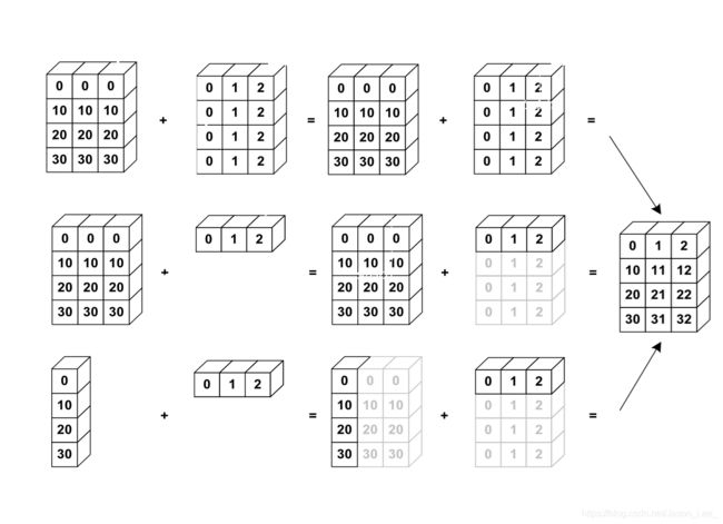
下图展示了简单地 Broadcasting 操作:
 |
|---|
| Broadcasting 操作示意图 第一行展示了两个维度信息相同 size=[4, 3] 的张量可以直接进行相加操作。 第二行中,一个 size=[4, 3] 和一个 size=[3] 的张量,这两个张量维度不同,不能直接相加,所以需要将第二个张量增加一个维度,并进行维度扩展后才可相加。 第三行中,一个 size=[4, 1] 和一个 size=[3] 的张量,这两个张量都需要进行修改后,才能进行相加。 第二、三行的操作就使用到了 Broadcasting 操作。 |
Broadcasting可以理解为自动扩展,也可直译为广播操作。 其可以实现:
- unsqueeze
实现维度增加, [ 32 , 1 , 1 ] ⇒ [ 1 , 32 , 1 , 1 ] [32, 1, 1]\Rightarrow[1, 32, 1, 1] [32,1,1]⇒[1,32,1,1],但是,只能在左侧插入维度。 - expand
实现维度扩展, [ 1 , 32 , 1 , 1 ] ⇒ [ 4 , 32 , 14 , 14 ] [1, 32, 1, 1]\Rightarrow[4, 32, 14, 14] [1,32,1,1]⇒[4,32,14,14] - without copying data
实现维度扩展时,不需要复制数据,可以节省内存。
关键点:
- 如果与目标张量维度不相同,在最前面增加维度;
- 进行维度扩展,使得新插入的第一个维度 size = 1 \text{size}=1 size=1 扩展成为与目标张量相同的 size \text{size} size
举个栗子:
对于目标张量 Feature map:size=[4, 32, 14, 14] ,我们想要使得 Bias:size=[32, 1, 1] 与 Feature map维度相匹配。那么,我们需要进行以下几个步骤:先在最前面增加一个维度,然后进行维度扩展,使得 Bias 维度信息与 Feature map 相一致。
Bias:size=[32, 1, 1]=>[1, 32, 1, 1]=>[4, 32, 14, 14]
注意:实际中,Bias 初始维度一般为 size=[32],但是 broadcasting 操作不能在后面增加维度,所以我们需要先使用 .unsqueeze() 操作手动增加维度,使得 Bias:size=[32]=>[32, 1, 1]。
完成以上操作以后,Feature map 与 Bias 的 shape 相同,才能进行相加。
Broadcasting操作的实际意义
以一个实际需求来分析一下 Broadcasting 操作的实际意义:
分数统计: 4个班级,每个班级32名学生,8门课,可是所有学生都考了55分,现在要为每位学生的每门成绩增加5分,使得所有学生都能够及格。
size = [Class Num, Student Num, Subject Num] = [4, 32, 8]
为每一名学生的每一门科目+5分;还可以通过设置 bias = [0, 5, 0, 7, 3, 0, 0, 0] 来为不同的科目增加不同的分数。此外,还可以通过设置 bias.shape = [Student Num, 1] 来为不同的同学增加不同的分数(独生子女、烈士子女加分优惠等)。
	# 分步完成
	In [7]: score = torch.full([4, 32, 8], 55, dtype=torch.float32)

	In [8]: score.shape
	Out[8]: torch.Size([4, 32, 8])

	In [9]: bias = torch.tensor([5])

	# 先将shape = [1]的bias增加维度为shape = [1, 1, 1],然后再使用expand_as将bias扩展为与score维度相同的shape = [2, 32, 8]
	In [11]: bias = bias.unsqueeze(0).unsqueeze(0).expand_as(score)

	In [12]: bias.shape
	Out[12]: torch.Size([4, 32, 8])

	In [13]: score = score + bias

	In [14]: score
	Out[14]:
	tensor([[[60., 60., 60.,  ..., 60., 60., 60.],
	         [60., 60., 60.,  ..., 60., 60., 60.],
	         ...,
	         [60., 60., 60.,  ..., 60., 60., 60.],
	         [60., 60., 60.,  ..., 60., 60., 60.]],

			...

	        [[60., 60., 60.,  ..., 60., 60., 60.],
	         [60., 60., 60.,  ..., 60., 60., 60.],
	         ...,
	         [60., 60., 60.,  ..., 60., 60., 60.],
	         [60., 60., 60.,  ..., 60., 60., 60.]]])

	# 通过自动的 Broadcasting 操作,直接相加
	In [16]: score = torch.full([4, 32, 8], 55, dtype=torch.float32)

	In [17]: bias = torch.tensor([5])

	In [18]: score = score + bias

	In [19]: score
	Out[19]:
	tensor([[[60., 60., 60.,  ..., 60., 60., 60.],
	         [60., 60., 60.,  ..., 60., 60., 60.],
	         ...,
	         [60., 60., 60.,  ..., 60., 60., 60.],
	         [60., 60., 60.,  ..., 60., 60., 60.]],

			...

	        [[60., 60., 60.,  ..., 60., 60., 60.],
	         [60., 60., 60.,  ..., 60., 60., 60.],
	         ...,
	         [60., 60., 60.,  ..., 60., 60., 60.],
	         [60., 60., 60.,  ..., 60., 60., 60.]]])
节省内存
在Broadcasting操作中,增加和扩展维度采用与expand相似的机制,不会直接复制数据内容,所以能够节省内存。如果使用repeat操作需要耗费内存:[4, 32, 8] => 1024;使用expand操作:[5.0] => 1。
实现Broadcasting操作的前提条件
实现Broadcasting操作的前提条件:不是任意形状的数组都可以通过 Broadcasting 操作进行相加。不同形状的数组相加需要满足以下要求:对于张量 a.shape = [ D 1 , D 2 , . . . , D m ] \text{a.shape}=[D_1, D_2, ...,D_m] a.shape=[D1,D2,...,Dm] 与张量 b.shape = [ D 1 , D 2 , . . . , D n ] \text{b.shape}=[D_1, D_2, ...,D_n] b.shape=[D1,D2,...,Dn] ,假设 m ≥ n m≥n m≥n,将二者维度从右向左对比,应该满足:
- 若 D m − k , D n − k ≠ 1 D_{m-k},D_{n-k}≠1 Dm−k,Dn−k=1,则必有 D m − k = D n − k D_{m-k}=D_{n-k} Dm−k=Dn−k;
- 若 D m − k ≠ D n − k D_{m-k}≠D_{n-k} Dm−k=Dn−k ,则必有 D m − k = 1 D_{m-k}=1 Dm−k=1 或 D n − k = 1 D_{n-k}=1 Dn−k=1;
- 其中, k = { 0 , 1 , 2 , . . . , n } k=\{0, 1, 2, ..., n\} k={ 0,1,2,...,n}。
如果张量 a 和张量 b 的维度不同,那么自动在小维度张量的左侧插入维度至与另一张量维度相同;然后,对于每一个size不同的维度,自动进行扩展expand操作至与另一张量相同。
举几个栗子:
- [4, 32, 14, 14]
给定数据维度[1, 32, 1, 1] => [4, 32, 14, 14] - [4, 32, 14, 14]
给定数据维度[14, 14] => [1, 1, 14, 14] => [4, 32, 14, 14] - [4, 32, 14, 14]
给定数据维度[2, 32, 14, 14],需要进行扩展操作的第0维size不为1,无法进行Broadcasting操作。
6.2 Tensor拼接与拆分
PyTorch中的几个实现拼接与拆分的API:
cat
concat,合并多个张量数组stack
合并操作split
按照长度进行拆分chunk
按照数量进行拆分
拼接
cat
torch.cat([a, b, c, ...], dim=) ,在列表中输入所有需要合并的张量,在dim=参数给定需要拼接的维度。下图给出了按照不同维度进行拼接的示意图:
| dim=0 | dim=1 |
|---|---|
 |
 |
学校分数统计,生成统一的成绩单:现在有两张成绩单,分别为 a.shape = [Class 1-4, Student Num, Scores],b.shape = [Class 5-7, Student Num, Scores],现在需要将 a、b 两张成绩单合并为1张。
	In [20]: a = torch.rand(4, 32, 8)

	In [21]: b = torch.rand(3, 32, 8)

	In [22]: total = torch.cat([a, b], dim=0)

	In [23]: total.shape
	Out[23]: torch.Size([7, 32, 8])
注意:除了给定的拼接维度以外,其余维度的size必须保持一致。
	In [31]: a = torch.rand(4, 3, 32, 32)

	In [32]: b = torch.rand(5, 3, 32, 32)

	In [33]: torch.cat([a, b], dim=0).shape
	Out[33]: torch.Size([9, 3, 32, 32])

	In [34]: b = torch.rand(4, 1, 32, 32)

	In [35]: torch.cat([a, b], dim=0).shape
	---------------------------------------------------------------------------
	RuntimeError                              Traceback (most recent call last)
	<ipython-input-35-08a943b55682> in <module>
	----> 1 torch.cat([a, b], dim=0).shape

	RuntimeError: Sizes of tensors must match except in dimension 0. Got 3 and 1 in dimension 1

	In [36]: torch.cat([a, b], dim=1).shape
	Out[36]: torch.Size([4, 4, 32, 32])

	In [37]: b = torch.rand(4, 3, 16, 32)

	In [39]: torch.cat([a, b], dim=2).shape
	Out[39]: torch.Size([4, 3, 48, 32])
stack
stack会完成与cat类似的操作,但是与cat不同的是,stack会创建一个新的维度。当需要合并的两个张量代表不同的含义时,需要使用到stack操作,以生成一个新的维度来区分这种不同的含义,比如合并两个不同班级的成绩单,生成一个新的维度来区分两个班级,[32, 8] + [32, 8] =>[64, 8]=>[2, 32, 8]。
	In [40]: a = torch.rand(4, 3, 16, 32)

	In [41]: b = torch.rand(4, 3, 16, 32)

	In [42]: torch.cat([a, b], dim=2).shape
	Out[42]: torch.Size([4, 3, 32, 32])

	In [43]: torch.stack([a, b], dim=2).shape
	Out[43]: torch.Size([4, 3, 2, 16, 32])

	In [44]: a1 = torch.rand(32, 8)

	In [45]: b1 = torch.rand(32, 8)

	In [46]: torch.stack([a1, b1], dim=0).shape
	Out[46]: torch.Size([2, 32, 8])
注意:使用stack操作的两个张量的所有维度信息必须相同,即必须要求 a.shape=b.shape。
	In [47]: a = torch.rand(4, 3, 16, 32)

	In [48]: b = torch.rand(4, 3, 32, 32)

	In [50]: torch.stack([a, b], dim=2).shape
	---------------------------------------------------------------------------
	RuntimeError                              Traceback (most recent call last)
	<ipython-input-50-7c9de06cfa6c> in <module>
	----> 1 torch.stack([a, b], dim=2).shape

	RuntimeError: stack expects each tensor to be equal size, but got [4, 3, 16, 32] at entry 0 and [4, 3, 32, 32] at entry 1

	In [51]: a = torch.rand(4, 3, 16, 32)

	In [52]: b = torch.rand(4, 2, 16, 32)

	In [53]: torch.stack([a, b], dim=2).shape
	---------------------------------------------------------------------------
	RuntimeError                              Traceback (most recent call last)
	<ipython-input-53-7c9de06cfa6c> in <module>
	----> 1 torch.stack([a, b], dim=2).shape

	RuntimeError: stack expects each tensor to be equal size, but got [4, 3, 16, 32] at entry 0 and [4, 2, 16, 32] at entry 1
切分
split:按照每块长度进行拆分,只要所有维度尺寸与拆分前的维度尺寸相同即可。
	In [58]: a.shape
	Out[58]: torch.Size([4, 3, 16, 32])

	In [59]: a = torch.rand(4, 3, 16, 32)

	In [60]: b = torch.rand(4, 3, 16, 32)

	In [61]: a1, a2 = a.split([2, 2], dim=0)

	In [62]: a1.shape, a2.shape
	Out[62]: (torch.Size([2, 3, 16, 32]), torch.Size([2, 3, 16, 32]))

	In [63]: a1, a2 = a.split([3, 1], dim=0)

	In [64]: a1.shape, a2.shape
	Out[64]: (torch.Size([3, 3, 16, 32]), torch.Size([1, 3, 16, 32]))

	In [66]: a1, a2, a3 = a.split([1, 2, 1], dim=0)

	In [67]: a1.shape, a2.shape, a3.shape
	Out[67]:
	(torch.Size([1, 3, 16, 32]),
	 torch.Size([2, 3, 16, 32]),
	 torch.Size([1, 3, 16, 32]))
chunk:按照分块数量进行拆分
torch.chunk(tensor, chunks, dim=n)
或者
a.chunk(chunks, dim=n)
chunks=n 代表切分成几部分;dim=n 代表要进行操作的维度索引。
注意(1):如果指定轴的元素个数被 chunks=n 除不尽,那么最后一块的元素个数减少;假设进行切分的维度尺寸为 n ,切分数量为 m,切分规则如下:
- 如果 n m \frac{n}{m} mn 为整数,则正好分为 m 份,每份的长度为 n m \frac{n}{m} mn ;
- 如果 n m \frac{n}{m} mn 为小数,则每份的长度向上取整为 ⌈ n m ⌉ \lceil\frac{n}{m}\rceil ⌈mn⌉ ,切分得到的张量个数为 ⌈ n ⌈ n / m ⌉ ⌉ \lceil\frac{n}{\lceil n/m \rceil}\rceil ⌈⌈n/m⌉n⌉
举个栗子: 如果要将维度尺寸为 4 的张量分割为 3 份,那么,每份的长度为 ⌈ 4 / 3 ⌉ = 2 \lceil4/3\rceil=2 ⌈4/3⌉=2 ,可以分为 4 / 2 = 2 4/2=2 4/2=2 ,不能得到期望的 3 份。
注意(2):根据以上切分规则,切分数量 chunks=n 可以设置为任意正整数,且不会报错,即使设置 chunks=n 非常大,也不会报错,而是直接按照以上规则进行切分。
	In [98]: a = torch.rand(4, 32, 16, 16)

	In [99]: aa, bb = a.chunk(2, dim=0)

	In [100]: aa.shape, bb.shape
	Out[100]: (torch.Size([2, 32, 16, 16]), torch.Size([2, 32, 16, 16]))

	In [102]: aa, bb, cc = a.chunk(3, dim=1)

	In [103]: aa.shape, bb.shape, cc.shape
	Out[103]:
	(torch.Size([4, 11, 16, 16]),
	 torch.Size([4, 11, 16, 16]),
	 torch.Size([4, 10, 16, 16]))
6.3 基本数学运算
常用的基本数学运算有:
- Add/minus/multiply/divide
- Matmul
- Pow
- Sqrt/rsqrt
- Round
注意:在PyTorch中,所有涉及两个元素运算的API都有两种实现形式,以加法为例:torch.add(a, b) 与 a.add(b)
add+/minus-/multiply×/divide÷
加减乘除运算在Pytorch中都有三种实现方法,一种是直接使用符号运算,另外两种是使用PyTorch提供的API。
	a = torch.rand(3, 4)
	b = torch.rand(4)

	# +
	c = a + b
	c = torch.add(a, b)
	c = a.add(b)

	# -
	c = a - b
	c = torch.sub(a, b)
	c = a.sub(b)

	# ×
	c = a * b
	c = torch.mul(a, b)
	c = a.mul(b)

	# ÷
	c = a / b
	c = torch.div(a, b)
	c = a.div(b)
matmul@
- 元素相乘(element-wise multiply):
* - 矩阵乘法:
matmultorch.mm仅适用于2D矩阵乘法;torch.matmul适用于任意维度矩阵乘法;@与torch.matmul相同。
	In [169]: a = torch.full([2, 2], 3, dtype=torch.float32)

	In [170]: b = torch.ones(2, 2)

	In [171]: torch.mm(a, b)
	Out[171]:
	tensor([[6., 6.],
	        [6., 6.]])

	In [172]: torch.matmul(a, b)
	Out[172]:
	tensor([[6., 6.],
	        [6., 6.]])

	In [173]: a @ b
	Out[173]:
	tensor([[6., 6.],
	        [6., 6.]])

	In [176]: a * b
	Out[176]:
	tensor([[3., 3.],
	        [3., 3.]])
神经网络线性层运算:
	In [177]: a = torch.rand(4, 784)

	In [178]: x = torch.rand(4, 784)

	# 在PyTorch中的书写习惯是:(channel-out, channel-in),所以此处将 w 写为 (512, 784)
	In [179]: w = torch.rand(512, 784)

	In [180]: (x @ w.t()).shape
	Out[180]: torch.Size([4, 512])
深度学习前向传播的过程就是一系列的矩阵相乘的过程,在神经网络中,输入x,参数weight、bias都为张量Tensor,其在神经网络中进行传播。
高维矩阵乘法规则
我们对于2D矩阵乘法的规则已经很熟悉了,对于 [ m , n ] × [ n , k ] ⇒ [ m , k ] [m, n]\times[n, k]\Rightarrow[m, k] [m,n]×[n,k]⇒[m,k] ,那么对于高维矩阵乘法的运算规则是什么样的?
以4D张量矩阵乘法为例: [ 4 , 3 , 28 , 64 ] × [ 4 , 3 , 64 , 32 ] [4, 3, 28, 64]\times[4, 3, 64, 32] [4,3,28,64]×[4,3,64,32] 在运算时,可以视为多个矩阵对并行相乘,即后面两维进行矩阵相乘,前面两位运算依从Broadcasting机制。即 [ 4 , 3 , 28 , 64 ] × [ 4 , 3 , 64 , 32 ] ⇒ [ 4 , 3 , 28 , 32 ] [4, 3, 28, 64]\times[4, 3, 64, 32]\Rightarrow[4, 3, 28, 32] [4,3,28,64]×[4,3,64,32]⇒[4,3,28,32]Broadcasting机制: [ 4 , 3 , 28 , 64 ] × [ 4 , 1 , 64 , 32 ] ⇒ [ 4 , 3 , 28 , 32 ] [4, 3, 28, 64]\times[4, 1, 64, 32]\Rightarrow[4, 3, 28, 32] [4,3,28,64]×[4,1,64,32]⇒[4,3,28,32]对于不符合Broadcasting机制的运算,同样会报错。
	In [182]: a = torch.rand(4, 3, 28, 64)

	In [183]: b = torch.rand(4, 3, 64, 32)

	In [184]: torch.mm(a, b)
	---------------------------------------------------------------------------
	RuntimeError                              Traceback (most recent call last)
	<ipython-input-184-d1e3b9067fee> in <module>
	----> 1 torch.mm(a, b)

	RuntimeError: matrices expected, got 4D, 4D tensors at C:\cb\pytorch_1000000000000\work\aten\src\TH/generic/THTensorMath.cpp:36

	In [185]: torch.matmul(a, b).shape
	Out[185]: torch.Size([4, 3, 28, 32])

	In [186]: b = torch.rand(4, 1, 64, 32)

	In [187]: torch.matmul(a, b).shape
	Out[187]: torch.Size([4, 3, 28, 32])

	In [188]: b = torch.rand(4, 64, 32)

	In [189]: torch.matmul(a, b).shape
	---------------------------------------------------------------------------
	RuntimeError                              Traceback (most recent call last)
	<ipython-input-189-8cd4f0e202ab> in <module>
	----> 1 torch.matmul(a, b).shape

	RuntimeError: The size of tensor a (3) must match the size of tensor b (4) at non-singleton dimension 1
power**/sqrt/rsqrt
乘方运算:
	In [190]: a = torch.full([2, 2], 3, dtype=torch.float32)

	In [191]: a.pow(2)
	Out[191]:
	tensor([[9., 9.],
	        [9., 9.]])

	In [192]: torch.pow(a, 2)
	Out[192]:
	tensor([[9., 9.],
	        [9., 9.]])

	In [193]: a ** 2
	Out[193]:
	tensor([[9., 9.],
	        [9., 9.]])
开方(Square root, sqrt)运算:
rsqrt()用于计算平方根的倒数
	In [195]: a = torch.full([2, 2], 3, dtype=torch.float32)

	In [196]: aa = a ** 2

	In [200]: aa.sqrt()
	Out[200]:
	tensor([[3., 3.],
	        [3., 3.]])

	In [201]: aa ** 0.5
	Out[201]:
	tensor([[3., 3.],
	        [3., 3.]])

	# rsqrt用于计算平方根的倒数
	In [202]: aa.rsqrt()
	Out[202]:
	tensor([[0.3333, 0.3333],
	        [0.3333, 0.3333]])
Exp/log/log2/log10
	In [203]: a = torch.exp(torch.ones(2, 2))

	In [204]: a
	Out[204]:
	tensor([[2.7183, 2.7183],
	        [2.7183, 2.7183]])

	In [205]: torch.log(a)
	Out[205]:
	tensor([[1., 1.],
	        [1., 1.]])

	In [206]: a.log()
	Out[206]:
	tensor([[1., 1.],
	        [1., 1.]])

	In [208]: a = torch.ones(2, 2)

	In [209]: a.exp()
	Out[209]:
	tensor([[2.7183, 2.7183],
	        [2.7183, 2.7183]])

	In [212]: torch.log2(torch.tensor([16, 16], dtype=torch.float32))
	Out[212]: tensor([4., 4.])

	In [213]: torch.log10(torch.tensor([100, 1000], dtype=torch.float32))
	Out[213]: tensor([2., 3.])
近似值Approximation
.flooe()、.ceil()向下、向上取整.round()四舍五入.trunc()、.frac()裁取整数部分、裁取小数部分
	In [216]: a = torch.tensor(3.14)

	In [217]: a.floor()
	Out[217]: tensor(3.)

	In [218]: a.ceil()
	Out[218]: tensor(4.)

	In [219]: a.floor(), a.ceil(), a.trunc(), a.frac()
	Out[219]: (tensor(3.), tensor(4.), tensor(3.), tensor(0.1400))

	In [220]: a.round()
	Out[220]: tensor(3.)

	In [221]: torch.round(torch.tensor(3.5))
	Out[221]: tensor(4.)
区间裁剪clamp
打印出梯度的2范数: w.grad.norm(2)
梯度弥散: 梯度很小,接近于0;
梯度爆炸: 梯度很大,一般梯度在10左右正常,100、1000就算很大了。
用的比较多的就是梯度裁剪(gradient clipping),常用于梯度弥散与梯度爆炸情况。
PyTorch提供的区间裁剪函数API如下:
	# %% 以下操作不直接对原始张量进行修改,需要再次对其进行赋值以执行修改。
	a.clamp(min, max)  # 将小于min的值全部设置为min,将大于max的值全部设置为max。
	a.clamp_min(min)  # 将小于min的值全部设置为min。
	a.clamp_max(max)  # 将大于max的值全部设置为max。

	#  %% 以下操作会直接对原始张量进行修改,功能与上述函数相同。
	a.clamp_(min, max)
	a.clamp_min_(min)
	a.clamp_max_(max)
举个栗子:
	In [222]: grad = torch.rand(2, 3) * 15

	In [223]: grad.max()
	Out[223]: tensor(11.3697)

	In [224]: grad.median()  # 中位数
	Out[224]: tensor(5.5786)

	In [226]: grad
	Out[226]:
	tensor([[ 6.9983,  5.5786,  3.2092],
	        [11.3697,  6.6925,  3.1998]])

	In [225]: grad.clamp(10)
	Out[225]:
	tensor([[10.0000, 10.0000, 10.0000],
	        [11.3697, 10.0000, 10.0000]])
对于实际网络参数使用 clamp 方法:
	for w in all_parameters:
		# 注意,一般是对w参数的梯度进行限幅,所以应该使用第二行代码
		w.clamp(10)  # 错误
		torch.clamp(w.grad, 10)  # 正确
6.4 Tensor统计属性
常用的统计属性有:
- norm
- mean, sum
- prod
- max, min, argmin, argmax
- kthvalue, topk
norm
范数作为一个统计信息,在训练神经网络时,有时候会使用norm查看参数梯度的范数值,以便对其进行约束。
注意(1):norm表示范数的含义,注意其与normalize归一化的区分,batch_norm表示批归一化。
归一化(Normalization)
标准化(Standardization)
正则化(Regularization)
注意(2):矩阵范数与向量范数的定义有些区别,需要注意区分:
- 1-Norm
∥ x ∥ 1 = ∑ i = 1 n ∣ a i ∣ \|x\|_1=\sum_{i=1}^n|a_i| ∥x∥1=∑i=1n∣ai∣
∥ A ∥ 1 = max 1 ≤ j ≤ n ∑ i = 1 n ∣ a i j ∣ \|A\|_1=\max_{1≤j≤n}\sum_{i=1}^n|a_{ij}| ∥A∥1=max1≤j≤n∑i=1n∣aij∣ - p-Norm
∥ x ∥ p = ( ∑ i = 1 n ∣ a i ∣ p ) 1 / p \|x\|_p=(\sum_{i=1}^n|a_i|^p)^{1/p} ∥x∥p=(∑i=1n∣ai∣p)1/p
∥ A ∥ p = ( ∑ i = 1 n ∑ j = 1 n a i j p ) 1 / p \|A\|_p=(\sum_{i=1}^n\sum_{j=1}^na_{ij}^p)^{1/p} ∥A∥p=(∑i=1n∑j=1naijp)1/p
PyTorch提供的Norm API:
a.norm(p, dim=n) 参数 p 给定要求的 p-Norm ,dim=n 表示对第 n 维度方求范数,比如 s h a p e = [ 2 , 4 ] shape=[2, 4] shape=[2,4] 对 dim=1 求范数,结果为 s h a p e = [ 2 ] shape=[2] shape=[2] 的张量。
	In [31]: a = torch.full([8], 1, dtype=torch.float32)

	In [32]: b = a.view(2, 4)

	In [33]: c = a.view(2, 2, 2)

	In [34]: a.norm(1), b.norm(1), c.norm(1)
	Out[34]: (tensor(8.), tensor(8.), tensor(8.))

	In [35]: a.norm(2), b.norm(2), c.norm(2)
	Out[35]: (tensor(2.8284), tensor(2.8284), tensor(2.8284))

	In [37]: b.norm(1, dim=1)
	Out[37]: tensor([4., 4.])

	In [38]: b.norm(2, dim=1)
	Out[38]: tensor([2., 2.])

	In [39]: b.norm(3, dim=1)
	Out[39]: tensor([1.5874, 1.5874])

	In [40]: c.norm(1, dim=0)
	Out[40]:
	tensor([[2., 2.],
	        [2., 2.]])

	In [41]: c.norm(2, dim=0)
	Out[41]:
	tensor([[1.4142, 1.4142],
	        [1.4142, 1.4142]])
mean, sum, min, max, prod
	In [43]: a = torch.arange(8).view(2, 4).float()

	In [44]: a
	Out[44]:
	tensor([[0., 1., 2., 3.],
	        [4., 5., 6., 7.]])

	In [45]: a.min(), a.max(), a.mean(), a.prod()  # prod累乘
	Out[45]: (tensor(0.), tensor(7.), tensor(3.5000), tensor(0.))

	In [46]: a.sum()
	Out[46]: tensor(28.)
argmin, argmax
	In [47]: a.argmax()  # 返回最大值的索引,注意,该索引为一维索引,会先将矩阵拉平,然后求索引。
	Out[47]: tensor(7)

	In [48]: a.argmin()  # 返回最小值的索引
	Out[48]: tensor(0)

	In [50]: a = torch.rand(4, 10)

	In [51]: a.argmax()
	Out[51]: tensor(26)

	In [52]: a.argmax(dim=1)  # 给定dim=n,会在第n维度进行最大值索引求取。
	Out[52]: tensor([7, 7, 6, 0])
统计属性的常见参数 dim, keepdim
dim=n 用于指定执行操作的维度
keepdim=True/False 当我们对 shape=[4, 10] 执行 a.max(dim=1) 操作时,输出结果为一个一维张量 shape=[4],使用了 keepdim=True 会使得结果保持与原张量相同的维度,即 shape=[4, 1]。
以一个照片10分类任务输出的结果为例,确定最符合的分类结果:
	In [55]: a = torch.rand(4, 10)

	In [56]: a.max(dim=1)
	Out[56]:
	torch.return_types.max(
	values=tensor([0.9037, 0.9758, 0.9524, 0.9960]),
	indices=tensor([3, 1, 9, 4]))  # 分类结果为:[3, 1, 9, 4]

	In [57]: a.max()
	Out[57]: tensor(0.9960)

	In [59]: value, index = a.max(dim=1, keepdim=True)

	In [60]: index.shape
	Out[60]: torch.Size([4, 1])

	In [61]: value, index = a.max(dim=1)

	In [62]: index.shape
	Out[62]: torch.Size([4])

	In [63]: a.argmax(dim=1, keepdim=True)
	Out[63]:
	tensor([[3],
	        [1],
	        [9],
	        [4]])
Top-k, k-th
Top-k
在ImageNet分类中,常用的一个度量标准为 top-5 Acc、top-1 Acc、top-k Acc,以一个10分类问题的预测结果来介绍一下top-k的含义:
对于10分类的结果: [ 0.4261 , 0.4415 , 0.8921 , 0.8390 , 0.3977 , 0.5558 , 0.8852 , 0.1716 , 0.6190 , 0.2788 ] [0.4261, 0.4415, 0.8921, 0.8390, 0.3977, 0.5558, 0.8852, 0.1716, 0.6190, 0.2788] [0.4261,0.4415,0.8921,0.8390,0.3977,0.5558,0.8852,0.1716,0.6190,0.2788],将每个类别的概率从大到小排序,返回概率值最高的前 k 个类别标签及其对应的概率值,如果这 k 个类别中包含了真实标签,那么就算分类正确,按照该标准得到的分类结果准确率称为 top-k Acc 。
a.topk(k, dim=n, largest=True/False) 其中的参数 k 指 top-k 中的 k 的大小,dim=n 指进行操作的维度,largest=True/False 设置为 True 指选取最大的 k 个,设置为 False 则选取最小的 k 个。
	In [68]: a = torch.rand(4, 10)

	In [69]: a.topk(3, dim=1)
	Out[69]:
	torch.return_types.topk(
	values=tensor([[0.8788, 0.8780, 0.7754],
	        [0.9091, 0.9048, 0.7810],
	        [0.9348, 0.8868, 0.7190],
	        [0.9917, 0.8903, 0.7897]]),
	indices=tensor([[3, 5, 8],
	        [5, 9, 1],
	        [6, 7, 5],
	        [7, 1, 5]]))

	In [70]: a.topk(3, dim=1, largest=False)
	Out[70]:
	torch.return_types.topk(
	values=tensor([[0.1048, 0.1696, 0.2655],
	        [0.0169, 0.2217, 0.2772],
	        [0.0377, 0.1624, 0.2808],
	        [0.1046, 0.2290, 0.3055]]),
	indices=tensor([[0, 9, 4],
	        [6, 4, 8],
	        [9, 8, 1],
	        [0, 8, 9]]))
k-th
a.kthvalue(k, dim=1) 从小到大排列,返回第 k 个值及其索引。
	In [71]: a.kthvalue(8, dim=1)
	Out[71]:
	torch.return_types.kthvalue(
	values=tensor([0.7754, 0.7810, 0.7190, 0.7897]),
	indices=tensor([8, 1, 5, 5]))

	In [72]: a.kthvalue(3)
	Out[72]:
	torch.return_types.kthvalue(
	values=tensor([0.2655, 0.2772, 0.2808, 0.3055]),
	indices=tensor([4, 8, 1, 9]))

	In [73]: a.kthvalue(3, dim=1)
	Out[73]:
	torch.return_types.kthvalue(
	values=tensor([0.2655, 0.2772, 0.2808, 0.3055]),
	indices=tensor([4, 8, 1, 9]))
常用的比较运算 Compare
>, >=, <, <=, !=, ==torch.eq(a, b)
	# >
	a > 0
	torch.gt(a, 0)

	# <
	a < 0
	torch.le(a, 0)

	# ==
	a == b
	torch.eq(a, b)  # 每个元素单独比较是否相等
	torch.equal(a, b)  # 所有元素都相等,返回True
举个栗子:
	In [74]: a = torch.randn(3, 5)

	In [75]: a
	Out[75]:
	tensor([[-0.8659,  1.1651,  1.0562,  0.8090, -0.7642],
	        [-0.9480, -0.2417, -0.4349,  0.1955,  0.5262],
	        [-1.6453, -1.3141, -1.4915,  0.0145, -0.4189]])

	In [76]: a > 0
	Out[76]:
	tensor([[False,  True,  True,  True, False],
	        [False, False, False,  True,  True],
	        [False, False, False,  True, False]])

	In [77]: torch.gt(a, 0)
	Out[77]:
	tensor([[False,  True,  True,  True, False],
	        [False, False, False,  True,  True],
	        [False, False, False,  True, False]])

	In [78]: a != 0
	Out[78]:
	tensor([[True, True, True, True, True],
	        [True, True, True, True, True],
	        [True, True, True, True, True]])

	In [80]: a = torch.rand(2, 3)

	In [81]: b = torch.ones(2, 3)

	In [82]: torch.eq(a, b)
	Out[82]:
	tensor([[False, False, False],
	        [False, False, False]])

	In [83]: torch.eq(a, a)
	Out[83]:
	tensor([[True, True, True],
	        [True, True, True]])

	In [84]: torch.equal(a, a)
	Out[84]: True
6.4 PyTorch高阶操作
本节主要讲解PyTorch中两个高阶操作:
where
给定条件,判断是否满足条件,以确定要执行的操作;gather
查表操作
where
torch.where(condition, a, b) 给定条件 condition 成立,则执行 a ,否则执行 b ,condition 可以给定多个条件,生成多个结果。举个栗子:
	In [99]: a = torch.tensor([[1, 0, 1], [0, 1, 1], [0, 1, 0]], dtype=torch.uint8)

	In [100]: a
	Out[100]:
	tensor([[1, 0, 1],
	        [0, 1, 1],
	        [0, 1, 0]], dtype=torch.uint8)

	In [101]: torch.where(a, torch.tensor(11), torch.tensor(00))
	Out[101]:
	tensor([[11,  0, 11],
	        [ 0, 11, 11],
	        [ 0, 11,  0]])
此外,还可以将 condition 和a、b设置为相同维度大小的张量,如下所示:
	In [102]: cond = torch.rand(2, 2)

	In [103]: cond
	Out[103]:
	tensor([[0.8441, 0.7396],
	        [0.3981, 0.9902]])

	In [104]: a = torch.zeros(2, 2)

	In [105]: b = torch.ones(2, 2)

	In [106]: torch.where(cond > 0.5, a, b)
	Out[106]:
	tensor([[0., 0.],
	        [1., 0.]])
以上功能也可以使用for循环实现,但是存在一个问题就是,如果使用for循环和if语句实现,那么该过程全部基于python语句,全部是在CPU上面实现的,无法实现GPU上的并行化运算,但是使用 torch.where(cond, a, b) 即可在GPU上运行。
gather
gather为收集之意,实现的是一个查表的过程,torch.gather(input, dim, index) 实现在指定的维度上收集数值。
应用场景: 一般神经网络输出的预测值一般使用索引作为相对标签,即只能设置为 [ 1 , 2 , . . . , n ] [1, 2, ..., n] [1,2,...,n] ,但是实际的标签Groundtruth可能是 [ 102 , 102 , . . . , 10 n ] [102, 102, ..., 10n] [102,102,...,10n] 等,所以就需要使用到 gather 函数进行查表操作:
	In [130]: pred = torch.rand(4, 10)

	In [131]: idx = pred.topk(3, dim=1)

	In [132]: idx
	Out[132]:
	torch.return_types.topk(
	values=tensor([[0.9927, 0.9791, 0.8770],
	        [0.9792, 0.9472, 0.9119],
	        [0.9871, 0.8949, 0.7825],
	        [0.8787, 0.8463, 0.6680]]),
	indices=tensor([[8, 6, 7],
	        [6, 7, 9],
	        [3, 5, 4],
	        [2, 1, 7]]))

	In [133]: pred_label = idx[1]

	In [134]: pred_label
	Out[134]:
	tensor([[8, 6, 7],
	        [6, 7, 9],
	        [3, 5, 4],
	        [2, 1, 7]])

	In [135]: ground_truth = torch.arange(10) + 100

	In [136]: ground_truth
	Out[136]: tensor([100, 101, 102, 103, 104, 105, 106, 107, 108, 109])

	In [139]: torch.gather(ground_truth.expand(4, 10), dim=1, index=pred_label.long())
	Out[139]:
	tensor([[108, 106, 107],
	        [106, 107, 109],
	        [103, 105, 104],
	        [102, 101, 107]])
本文仅为笔者PyTorch学习笔记,部分图文来源于网络,若有侵权,联系即删。
Reference
https://study.163.com/course/introduction/1208894818.htm